Week 6

Model Diagnostics and Results Reporting

Week Learning Objectives

By the end of this module, you will be able to

• Describe the major assumptions in basic multilevel models
• Conduct analyses to decide whether cluster means and random slopes should be included
• Use graphical tools to diagnose assumptions of linearity, homoscedasticity (equal variance), and normality
• Solve some basic convergence issues
• Report results of a multilevel analysis based on established guidelines

Task Lists

1. Review the resources (lecture videos and slides)
2. Complete the assigned readings
   • Snijders & Bosker ch 10
   • Meteyard & Davies (2020; to be shared on Slack)
   • McCoach (2019 chapter) (USC SSO required)
3. Attend the Thursday session and participate in the class exercise
4. Complete Homework 6

Lecture

Slides

You can view and download the slides here: HTML PDF

Model Diagnostics

Check your learning: Homoscedasticity means

Equal variance of errors
Each cluster has the same mean
The model resembles the data

Assumptions of a Multilevel Model

Note: \(\mathrm{E}(Y)\) can also be written as \(\hat Y\), the predicted value of \(Y\) based on the predictor values.

The linear model is also flexible as it can allow predictors that are curvillinear terms, such as \(Y = b_0 + b_1 X_1 + b_2 X_1^2\), or \(Y = b_0 + b_1 \log(X_1)\), or more generally \[Y = b_0 + \sum_{i}^p b_i f(x_1, x_2, \ldots)\] The “linear” part in a linear model actually means that \(Y\) is a linear function of the coefficients \(b_1, b_2, \ldots\).

The second functional form in the slide, however, is a truly nonlinear function.

Check your learning: Which of the following is NOT a linear model?

Y = X1 + X2
Y = b0 + b1 * X1 + b2 * X2 + b3 * X1 * X2
Y = b0 * exp(b1 * X1 + b2 * X2)

Check your learning: What is implied when the model specifies that the variance of \(u_{0j}\) is \(\tau^2_0\)?

The intercept variance is constant across different clusters
The slope is different across clusters
The intercept variance is different for different types of schools

Remember the “LINES”

Check your learning: What does “I” stand for?

Increasing trend of outcome
Independence of errors
Independence of predictors

Check your learning: What is shown in a marginal model plot?

Whether the model shows a linear association between a predictor and the outcome
Whether the model-implied association is similar to the model-free (i.e., marginal) association
Whether the margin of error in the model is small enough

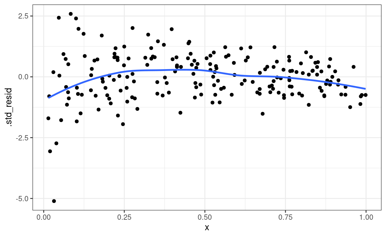
Check your learning: Which assumption(s) are likely violated in the following plot?

linearity
equal variance of errors
normality
linearity and equal variance of errors

Additional issues

• Outliers/influential observations
  • Check coding error
  • Don’t drop outliers unless you adjust the standard errors accordingly, or use robust models
• Reliability (e.g., \(\alpha\) coefficient)
  • Reliability may be high at one level but low at another level
  • See Lai (2021, doi: 10.1037/met0000287) for level-specific reliability
    • You can use the multilevel_alpha() function from https://github.com/marklhc/mcfa_reliability_supp/blob/master/multilevel_alpha.R

Handling Convergence Issues

See R codes for this week

Reporting Results