\[ \newcommand{\bv}[1]{\boldsymbol{\mathbf{#1}}} \]
Click here to download the Rmd file: week3-random-intercept-model.Rmd
Load Packages and Import Data
You can use the message=FALSE option to suppress the
package loading messages
# To install a package, run the following ONCE (and only once on your computer)
# install.packages("psych")
library(here)  # makes reading data more consistent
library(tidyverse)  # for data manipulation and plotting
library(haven)  # for importing SPSS/SAS/Stata data
library(lme4)  # for multilevel analysis
library(lattice)  # for dotplot (working with lme4)
library(sjPlot)  # for plotting effects
library(MuMIn)  # for computing r-squared
library(r2mlm)  # for computing r-squared
library(broom.mixed)  # for summarizing results
library(modelsummary)  # for making tables
theme_set(theme_bw())  # Theme; just my personal preference
In R, there are many packages for multilevel modeling, two of the
most common ones are the lme4 package and the
nlme package. In this note I will show how to run different
basic multilevel models using the lme4 package, which is
newer. However, some of the models, like unstructured covariance
structure, will need the nlme package or other packages
(like the brms and the rstanarm packages with
Bayesian estimation).
Import Data
First, download the data from https://github.com/marklhc/marklai-pages/raw/master/data_files/hsball.sav.
We’ll import the data in .sav format using the read_sav()
function from the haven package.
# Read in the data (pay attention to the directory)
hsball <- read_sav(here("data_files", "hsball.sav"))
hsball  # print the data
># # A tibble: 7,185 × 11
>#    id    minority female    ses mathach  size sector pracad disclim
>#    <chr>    <dbl>  <dbl>  <dbl>   <dbl> <dbl>  <dbl>  <dbl>   <dbl>
>#  1 1224         0      1 -1.53    5.88    842      0   0.35    1.60
>#  2 1224         0      1 -0.588  19.7     842      0   0.35    1.60
>#  3 1224         0      0 -0.528  20.3     842      0   0.35    1.60
>#  4 1224         0      0 -0.668   8.78    842      0   0.35    1.60
>#  5 1224         0      0 -0.158  17.9     842      0   0.35    1.60
>#  6 1224         0      0  0.022   4.58    842      0   0.35    1.60
>#  7 1224         0      1 -0.618  -2.83    842      0   0.35    1.60
>#  8 1224         0      0 -0.998   0.523   842      0   0.35    1.60
>#  9 1224         0      1 -0.888   1.53    842      0   0.35    1.60
># 10 1224         0      0 -0.458  21.5     842      0   0.35    1.60
># # … with 7,175 more rows, and 2 more variables: himinty <dbl>,
># #   meanses <dbl>
Run the Random Intercept Model
Model equations
Lv-1: \[\text{mathach}_{ij} = \beta_{0j} + e_{ij}\] where \(\beta_{0j}\) is the population mean math achievement of the \(j\)th school, and \(e_{ij}\) is the level-1 random error term for the \(i\)th individual of the \(j\)th school.
Lv-2: \[\beta_{0j} = \gamma_{00} + u_{0j}\] where \(\gamma_{00}\) is the grand mean, and \(u_{0j}\) is the deviation of the mean of the \(j\)th school from the grand mean.
Running the model in R
The lme4 package require input in the format of
outcome ~ fixed + (random | cluster ID)For our data, the combined equation is \[\text{mathach}_{ij} = \gamma_{00} + u_{0j} + e_{ij}, \] which we can explicitly write \[\color{red}{\text{mathach}}_{ij} = \color{green}{\gamma_{00} (1)} + \color{blue}{u_{0j} (1)} + e_{ij}. \] With that, we can see
- outcome =
mathach, - fixed =
1, - random =
1, and - cluster ID =
id.
Thus the following syntax:
# outcome = mathach
# fixed = gamma_{00} * 1
# random = u_{0j} * 1, with j indexing school id
ran_int <- lmer(mathach ~ 1 + (1 | id), data = hsball)
# Summarize results
summary(ran_int)
># Linear mixed model fit by REML ['lmerMod']
># Formula: mathach ~ 1 + (1 | id)
># Data: hsball
>#
># REML criterion at convergence: 47117
>#
># Scaled residuals:
># Min 1Q Median 3Q Max
># -3.0631 -0.7539 0.0267 0.7606 2.7426
>#
># Random effects:
># Groups Name Variance Std.Dev.
># id (Intercept) 8.61 2.93
># Residual 39.15 6.26
># Number of obs: 7185, groups: id, 160
>#
># Fixed effects:
># Estimate Std. Error t value
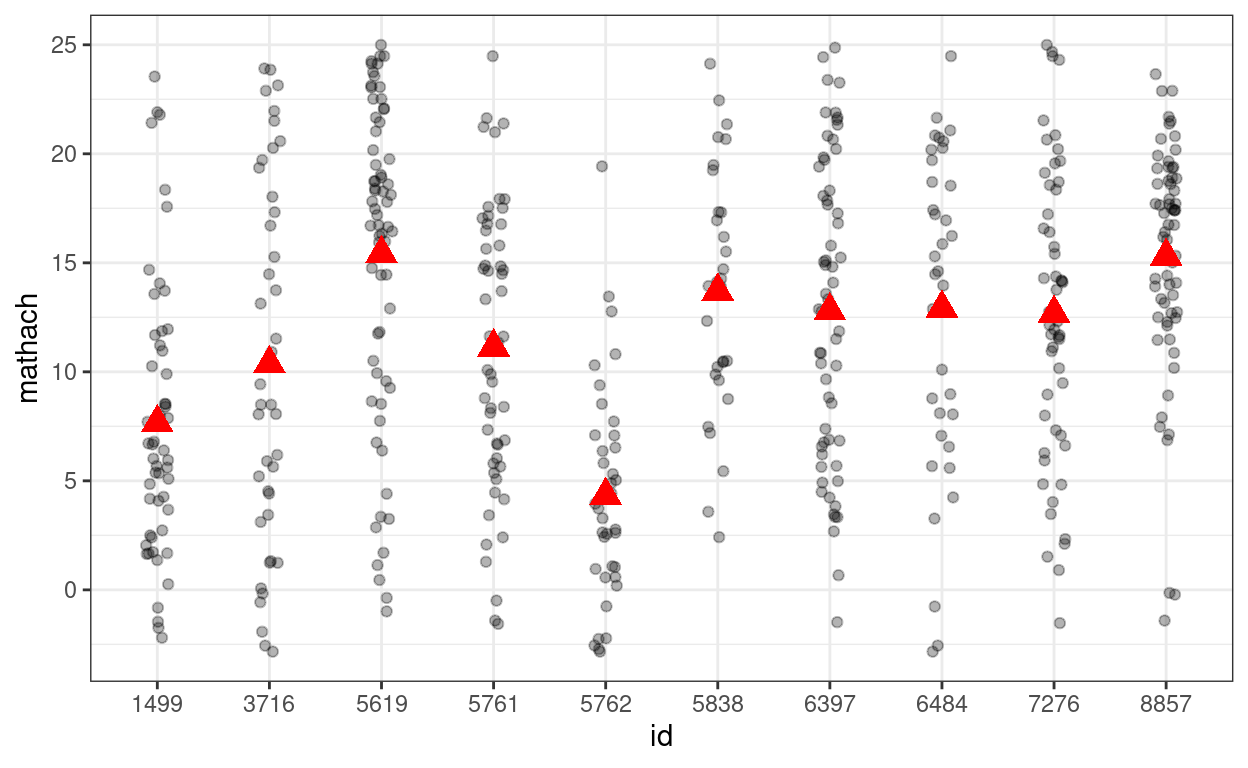
># (Intercept) 12.637 0.244 51.7Showing the variations across (a subset of) schools
# Randomly select 10 school ids
random_ids <- sample(unique(hsball$id), size = 10)
(p_subset <- hsball %>%
    filter(id %in% random_ids) %>%  # select only 10 schools
    ggplot(aes(x = id, y = mathach)) +
    geom_jitter(height = 0, width = 0.1, alpha = 0.3) +
    # Add school means
    stat_summary(
      fun = "mean",
      geom = "point",
      col = "red",
      shape = 17,
      # use triangles
      size = 4
    )  # make them larger
)
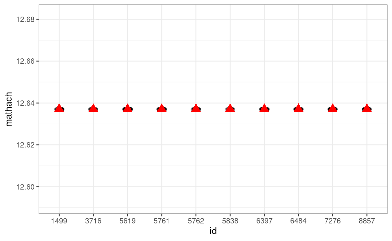
Simulating data based on the random intercept model
\[Y_{ij} = \gamma_{00} + u_{0j} + e_{ij},\]
gamma00 <- 12.6370
tau0 <- 2.935
sigma <- 6.257
num_students <- nrow(hsball)
num_schools <- length(unique(hsball$id))
# Simulate with only gamma00 (i.e., tau0 = 0 and sigma = 0)
simulated_data1 <- tibble(
  id = hsball$id,
  mathach = gamma00
)
# Show data with no variation
# The `%+%` operator is use to substitute with a different data set
p_subset %+%
  (simulated_data1 %>%
     filter(id %in% random_ids))
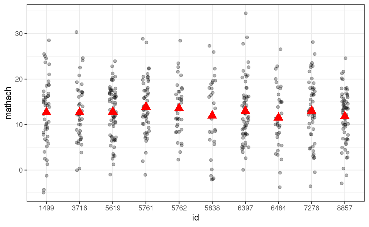
# Simulate with gamma00 + e_ij (i.e., tau0 = 0)
simulated_data2 <- tibble(
  id = hsball$id,
  mathach = gamma00 + rnorm(num_students, sd = sigma)
)
# Show data with no school-level variation
p_subset %+%
  (simulated_data2 %>%
     filter(id %in% random_ids))
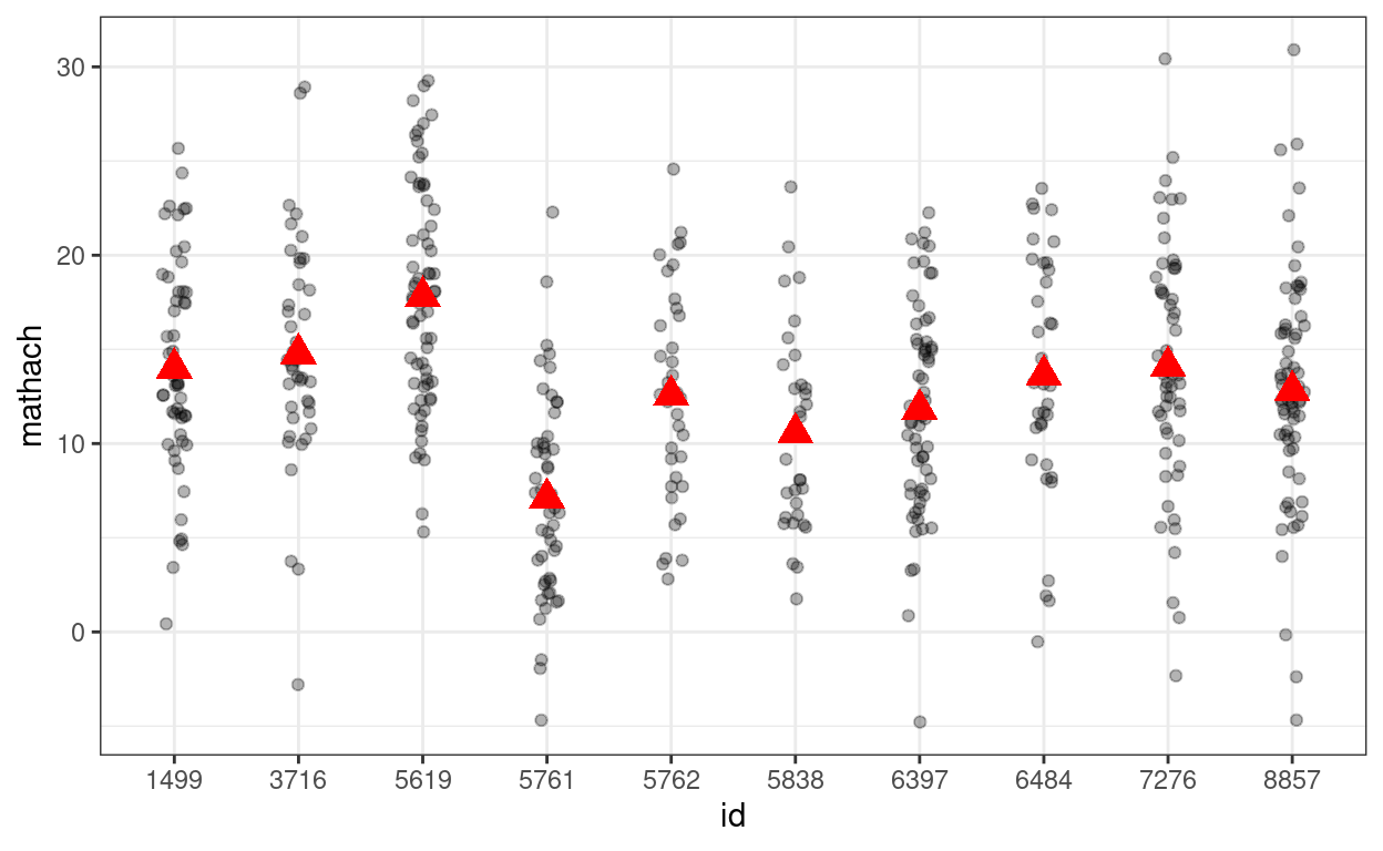
# Simulate with gamma00 + u_0j + e_ij
# First, obtain group indices that starts from 1 to 160
group_idx <- group_by(hsball, id) %>% group_indices()
# Then simulate 160 u0j
u0j <- rnorm(num_schools, sd = tau0)
simulated_data3 <- tibble(
  id = hsball$id,
  mathach = gamma00 +
    u0j[group_idx] +  # expand the u0j's from 160 to 7185
    rnorm(num_students, sd = sigma)
)
# Show data with both school and student variations
p_subset %+%
  (simulated_data3 %>%
     filter(id %in% random_ids))
The handy simulate() function can also be used to
simulate the data
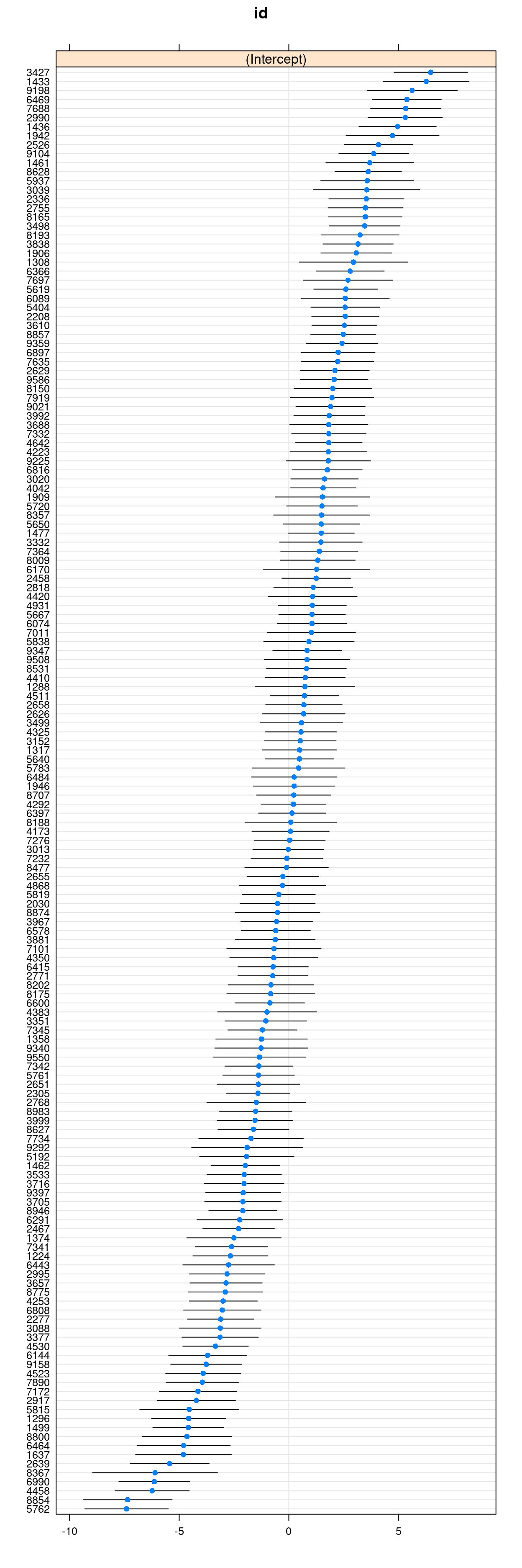
Plotting the random effects (i.e., \(u_{0j}\))
You can easily plot the estimated school means (also called BLUP,
best linear unbiased predictor, or the empirical Bayes (EB) estimates,
which are different from the mean of the sample observations for a
particular school) using the lattice package:
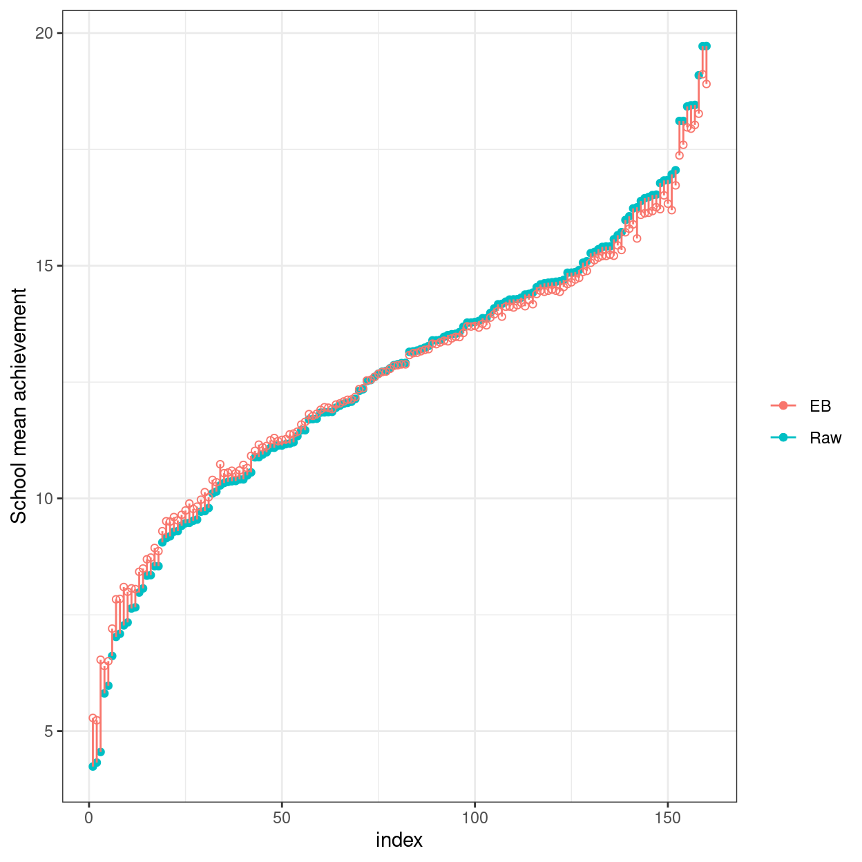
Here’s a plot showing the sample schools means (with no borrowing of information) vs. the EB means (borrowing information).
# Compute raw school means and EB means
hsball %>%
  group_by(id) %>%
  # Raw means
  summarise(mathach_raw_means = mean(mathach)) %>%
  arrange(mathach_raw_means) %>%  # sort by the means
  # EB means (the "." means using the current data)
  mutate(mathach_eb_means = predict(ran_int, .),
         index = row_number()) %>%  # add row number as index for plotting
  ggplot(aes(x = index, y = mathach_raw_means)) +
  geom_point(aes(col = "Raw")) +
  # Add EB means
  geom_point(aes(y = mathach_eb_means, col = "EB"), shape = 1) +
  geom_segment(aes(x = index, xend = index,
                   y = mathach_eb_means, yend = mathach_raw_means,
                   col = "EB")) +
  labs(y = "School mean achievement", col = "")
Intraclass correlations
variance_components <- as.data.frame(VarCorr(ran_int))
between_var <- variance_components$vcov[1]
within_var <- variance_components$vcov[2]
(icc <- between_var / (between_var + within_var))
># [1] 0.1804# 95% confidence intervals (require installing the bootmlm package)
# if (!require("devtools")) {
# install.packages("devtools")
# }
# devtools::install_github("marklhc/bootmlm")
bootmlm:::prof_ci_icc(ran_int)
>#  2.5 % 97.5 %
># 0.1472 0.2210
Adding Lv-2 Predictors
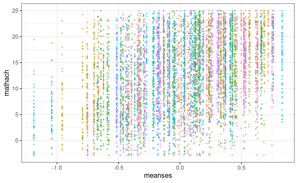
We have one predictor, meanses, in the fixed part.
hsball %>%
  ggplot(aes(x = meanses, y = mathach, col = id)) +
  geom_point(alpha = 0.5, size = 0.5) +
  guides(col = "none")
Model Equation
Lv-1:
\[\text{mathach}_{ij} = \beta_{0j} + e_{ij}\]
Lv-2:
\[\beta_{0j} = \gamma_{00} + \gamma_{01}
\text{meanses}_j + u_{0j}\] where \(\gamma_{00}\) is the grand
intercept, \(\gamma_{10}\) is
the regression coefficient of meanses that represents the
expected difference in school mean achievement between two schools with
one unit difference in meanses, and and \(u_{0j}\) is the deviation of the mean of
the \(j\)th school from the grand
mean.
># Linear mixed model fit by REML ['lmerMod']
># Formula: mathach ~ meanses + (1 | id)
>#    Data: hsball
>#
># REML criterion at convergence: 46961
>#
># Scaled residuals:
>#     Min      1Q  Median      3Q     Max
># -3.1348 -0.7526  0.0241  0.7677  2.7850
>#
># Random effects:
>#  Groups   Name        Variance Std.Dev.
>#  id       (Intercept)  2.64    1.62
>#  Residual             39.16    6.26
># Number of obs: 7185, groups:  id, 160
>#
># Fixed effects:
>#             Estimate Std. Error t value
># (Intercept)   12.649      0.149    84.7
># meanses        5.864      0.361    16.2
>#
># Correlation of Fixed Effects:
>#         (Intr)
># meanses -0.004
# Likelihood-based confidence intervals for fixed effects
# `parm = "beta_"` requests confidence intervals only for the fixed effects
confint(m_lv2, parm = "beta_")
># 2.5 % 97.5 %
># (Intercept) 12.357 12.942
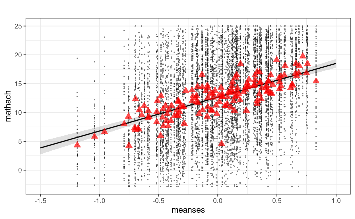
># meanses 5.156 6.572The 95% confidence intervals (CIs) above showed the uncertainty
associated with the estimates. Also, as the 95% CI for
meanses does not contain zero, there is evidence for the
positive association of SES and mathach at the school
level.
sjPlot::plot_model(m_lv2, type = "pred", terms = "meanses",
                   show.data = TRUE, title = "",
                   dot.size = 0.5) +
  # Add the group means
  stat_summary(data = hsball, aes(x = meanses, y = mathach),
               fun = mean, geom = "point",
               col = "red",
               shape = 17,
               # use triangles
               size = 3,
               alpha = 0.7)
Proportion of variance predicted
We will use the \(R^2\) statistic proposed by Nakagawa, Johnson & Schielzeth (2017) to obtain an \(R^2\) statistic. There are multiple versions of \(R^2\) in the literature, but personally I think this \(R^2\) avoids many of the problems in other variants and is most meaningful to interpret. Note that I only interpret the marginal \(R^2\).
# Generally, you should use the marginal R^2 (R2m) for the variance predicted by
# your predictors (`meanses` in this case).
MuMIn::r.squaredGLMM(m_lv2)
>#         R2m    R2c
># [1,] 0.1233 0.1787
An alternative, more comprehensive approach is by Rights & Sterba
(2019, Psychological Methods, https://doi.org/10.1037/met0000184), with the
r2mlm package
r2mlm::r2mlm(m_lv2)
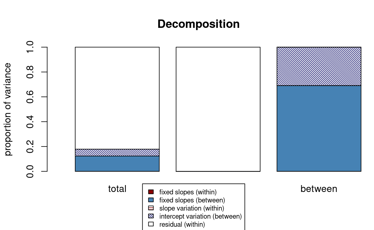
># $Decompositions
>#                 total              within between
># fixed, within   0                  0      NA
># fixed, between  0.123334641367122  NA     0.690248683624938
># slope variation 0                  0      NA
># mean variation  0.0553468169145697 NA     0.309751316375062
># sigma2          0.821318541718308  1      NA
>#
># $R2s
>#     total              within between
># f1  0                  0      NA
># f2  0.123334641367122  NA     0.690248683624938
># v   0                  0      NA
># m   0.0553468169145697 NA     0.309751316375062
># f   0.123334641367122  NA     NA
># fv  0.123334641367122  0      NA
># fvm 0.178681458281692  NA     NA
Note the fixed, between number in the total
column is the same as the one from MuMIn::r.squaredGLMM().
Including school means of SES in the model accounted for about 12% of
the total variance of math achievement.
Comparing to OLS regression
Notice that the standard error with regression is only half of that with MLM.
m_lm <- lm(mathach ~ meanses, data = hsball)
msummary(list("MLM" = m_lv2,
              "Linear regression" = m_lm))
| MLM | Linear regression | |
|---|---|---|
| (Intercept) | 12.649 | 12.713 |
| (0.149) | (0.076) | |
| meanses | 5.864 | 5.717 |
| (0.361) | (0.184) | |
| sd__(Intercept) | 1.624 | |
| sd__Observation | 6.258 | |
| Num.Obs. | 7185 | 7185 |
| R2 | 0.118 | |
| R2 Adj. | 0.118 | |
| AIC | 46969.3 | 47202.4 |
| BIC | 46996.8 | 47223.0 |
| Log.Lik. | −23480.642 | −23598.190 |
| F | 962.329 | |
| RMSE | 6.46 | |
| REMLcrit | 46961.285 |