Week Learning Objectives
By the end of this module, you will be able to
- Describe conceptually what likelihood function and maximum likelihood estimation are
- Describe the differences between maximum likelihood and restricted maximum likelihood
- Conduct statistical tests for fixed effects
- Test fixed effects using the F-test with the small-sample correction when the number of clusters is small
- Use the likelihood ratio test to test random slopes
Task Lists
- Review the resources (lecture videos and slides)
- Complete the assigned readings
- Snijders & Bosker ch 4.7, 6
- Attend the Thursday session and participate in the class exercise
- Complete Homework 5
- (Optional) Fill out the early/mid-semester feedback survey on Blackboard
Lecture
Slides
You can view and download the slides here: HTML PDF
Estimation Methods
Check your learning: The values you obtained from MLM software (e.g.,
lme4) are
Maximum likelihood
Check your learning: Using R, verify that, if \(\mu = 10\) and \(\sigma = 8\) for a normally distributed population, the probability (joint density) of getting students with scores of 23, 16, 5, 14, 7.
Check your learning: Using the principle of maximum likelihood, the best estimate for a parameter is one that
Thought exercise: Because a probability is less than 1, the logarithm of it will be a negative number. By that logic, if the log-likelihood is -16.5 with \(N = 5\), what should it be with a larger sample size (e.g., \(N = 50\))?
More about maximum likelihood estimation
If \(\sigma\) is not known, the maximum likelihood estimate is \[\hat \sigma = \sqrt{\frac{\sum_{i = 1}^N (Y_i - \bar X)^2}{N}},\] which uses \(N\) in the denominator instead of \(N - 1\). Because of this, in small sample, maximum likelihood estimate tends to be biased, meaning that on average it tends to underestimate the population variance.
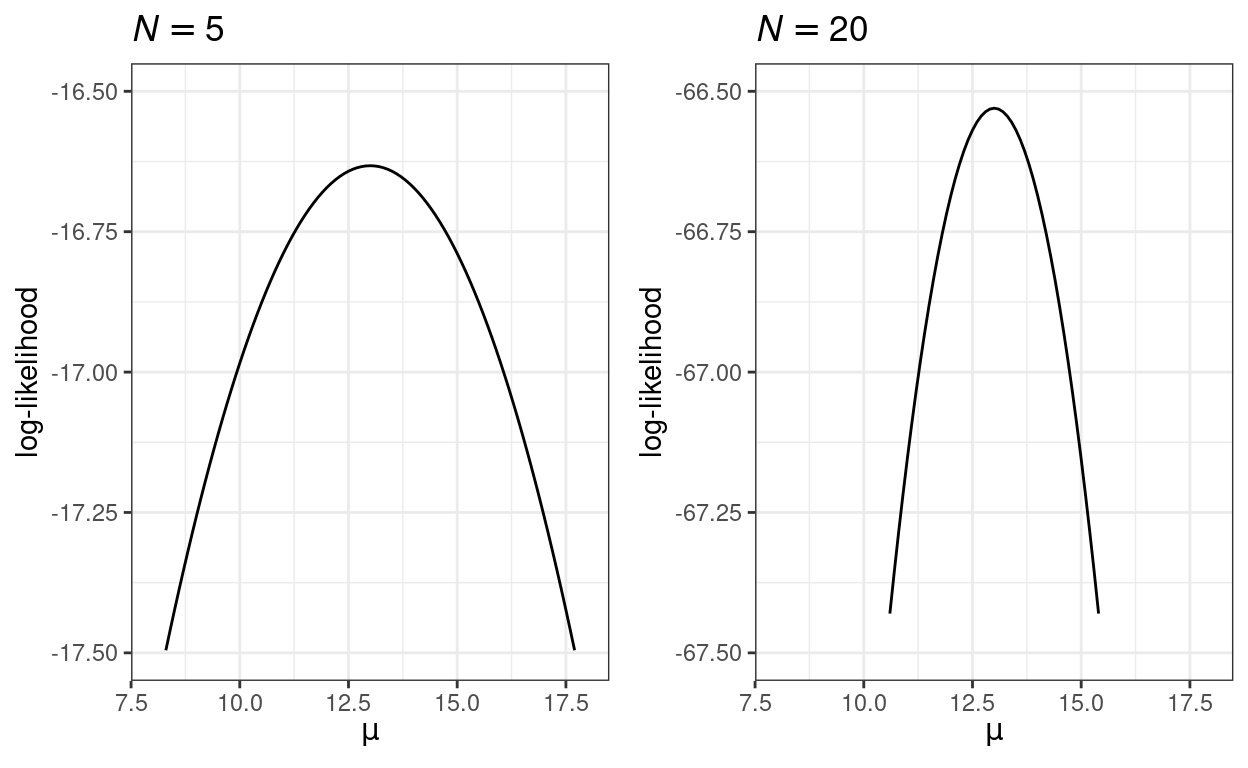
One useful property of maximum likelihood estimation is that the standard error can be approximated by the inverse of the curvature of the likelihood function at the peak. The two graphs below show that with a larger sample, the likelihood function has a higher curvature (i.e., steeper around the peak), which results in a smaller estimated standard error.
Estimation methods for MLM
Check your learning: The deviance is
Testing
Likelihood ratio test (LRT) for fixed effects
The LRT has been used widely across many statistical methods, so it’s useful to get familiar to doing it by hand (as it may not be available in all software in all procedures).
Practice yourself: Consider the two models below
| Model 1 | Model 2 | |
|---|---|---|
| (Intercept) | 12.650 | 12.662 |
| (0.148) | (0.148) | |
| meanses | 5.863 | 3.674 |
| (0.359) | (0.375) | |
| sd__(Intercept) | 1.610 | 1.627 |
| sd__Observation | 6.258 | 6.084 |
| ses | 2.191 | |
| (0.109) | ||
| Num.Obs. | 7185 | 7185 |
| AIC | 46967.1 | 46573.8 |
| BIC | 46994.6 | 46608.2 |
| Log.Lik. | −23479.554 | −23281.902 |
Using R and the pchisq() function, what is the \(\chi^2\) (or X2) test statistic and the
\(p\) value for the fixed effect
coefficient for ses?
\(F\) test with small-sample correction
Check your learning: From the results below, what is the test
statistic and the \(p\) value for the
fixed effect coefficient for meanses?
Type III Analysis of Variance Table with Kenward-Roger's method
        Sum Sq Mean Sq NumDF DenDF F value  Pr(>F)
meanses    324     324     1    16    9.96  0.0063 **
ses       1874    1874     1   669   57.53 1.1e-13 ***
---
Signif. codes:  0 '***' 0.001 '**' 0.01 '*' 0.05 '.' 0.1 ' ' 1
For more information on REML and K-R, check out
- McNeish, D. (2017). Small sample methods for multilevel modeling: A colloquial elucidation of REML and the Kenward-Roger correction.
LRT for random slope variance
Check your learning: When testing whether the variance of a random slope term is zero, what needs to be done?
Multilevel bootstrap