\[ \newcommand{\bv}[1]{\boldsymbol{\mathbf{#1}}} \]
Click here to download the Rmd file: week8-longitudinal-1.Rmd
Load Packages and Import Data
# To install a package, run the following ONCE (and only once on your computer)
# install.packages("psych")
library(here)  # makes reading data more consistent
library(tidyverse)  # for data manipulation and plotting
library(haven)  # for importing SPSS/SAS/Stata data
library(lme4)  # for multilevel analysis
library(glmmTMB)  # for longitudinal analysis
library(modelsummary)  # for making tables
library(interactions)  # for interaction plots
theme_set(theme_bw())  # Theme; just my personal preference
# Read in the data from gitHub (need Internet access)
curran_wide <- read_sav("https://github.com/MultiLevelAnalysis/Datasets-third-edition-Multilevel-book/raw/master/chapter%205/Curran/CurranData.sav")
# Make id a factor
curran_wide  # print the data
># # A tibble: 405 × 15
>#       id anti1 anti2 anti3 anti4 read1 read2 read3 read4    kidgen
>#    <dbl> <dbl> <dbl> <dbl> <dbl> <dbl> <dbl> <dbl> <dbl> <dbl+lbl>
>#  1    22     1     2    NA    NA   2.1   3.9  NA    NA    0 [girl]
>#  2    34     3     6     4     5   2.1   2.9   4.5   4.5  1 [boy]
>#  3    58     0     2     0     1   2.3   4.5   4.2   4.6  0 [girl]
>#  4   122     0     3     1     1   3.7   8    NA    NA    1 [boy]
>#  5   125     1     1     2     1   2.3   3.8   4.3   6.2  0 [girl]
>#  6   133     3     4     3     5   1.8   2.6   4.1   4    1 [boy]
>#  7   163     5     4     5     5   3.5   4.8   5.8   7.5  1 [boy]
>#  8   190     0    NA    NA     0   2.9   6.1  NA    NA    0 [girl]
>#  9   227     0     0     2     1   1.8   3.8   4    NA    0 [girl]
># 10   248     1     2     2     0   3.5   5.7   7     6.9  0 [girl]
># # … with 395 more rows, and 5 more variables: momage <dbl>,
># #   kidage <dbl>, homecog <dbl>, homeemo <dbl>, nmis <dbl>
Wide to Long
To perform multilevel analysis, we need to restructure the data from a wide format to a long format:
# Using the new `tidyr::pivot_longer()` function
curran_long <- curran_wide %>%
  pivot_longer(
    c(anti1:anti4, read1:read4),  # variables that are repeated measures
    # Convert 8 columns to 3: 2 columns each for anti/read (.value), and
    # one column for time
    names_to = c(".value", "time"),
    # Extract the names "anti"/"read" from the names of the variables for the
    # value columns, and then the number to the "time" column
    names_pattern = "(anti|read)([1-4])",
    # Convert the "time" column to integers
    names_transform = list(time = as.integer)
  )
curran_long %>%
  select(id, anti, read, time, everything())
># # A tibble: 1,620 × 10
>#       id  anti  read  time  kidgen momage kidage homecog homeemo  nmis
>#    <dbl> <dbl> <dbl> <int> <dbl+l>  <dbl>  <dbl>   <dbl>   <dbl> <dbl>
>#  1    22     1   2.1     1 0 [gir…     28   6.08      13      10     4
>#  2    22     2   3.9     2 0 [gir…     28   6.08      13      10     4
>#  3    22    NA  NA       3 0 [gir…     28   6.08      13      10     4
>#  4    22    NA  NA       4 0 [gir…     28   6.08      13      10     4
>#  5    34     3   2.1     1 1 [boy]     28   6.83       9       9     0
>#  6    34     6   2.9     2 1 [boy]     28   6.83       9       9     0
>#  7    34     4   4.5     3 1 [boy]     28   6.83       9       9     0
>#  8    34     5   4.5     4 1 [boy]     28   6.83       9       9     0
>#  9    58     0   2.3     1 0 [gir…     28   6.5        9       6     0
># 10    58     2   4.5     2 0 [gir…     28   6.5        9       6     0
># # … with 1,610 more rows
Data Exploration
curran_long %>%
    select(time, kidage, homecog, anti, read) %>%
    psych::pairs.panels(jiggle = TRUE, factor = 0.5, ellipses = FALSE,
                        cex.cor = 1, cex = 0.5)
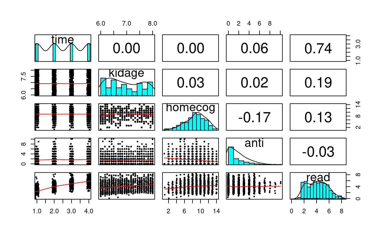
What distinguishes longitudinal data from usual cross-sectional multilevel data is the temporal ordering. In the example of students nested within schools, we don’t say that student 1 is naturally before student 2, and it doesn’t really matter if one just reorder the students. However, in longitudinal data such temporal sequence is very important, and we cannot simply rearrange the observation at time 2 to be at time 1. A related concern is the presence of autocorrelation, with which observations closer in time will be more similar to each other.
Spaghetti Plot
# Plotting
p1 <- ggplot(curran_long, aes(x = time, y = read)) +
  geom_point() +
  geom_line(aes(group = id)) +  # add lines to connect the data for each person
  # add a mean trajectory
  stat_summary(fun = "mean", col = "red", size = 1, geom = "line")
p1
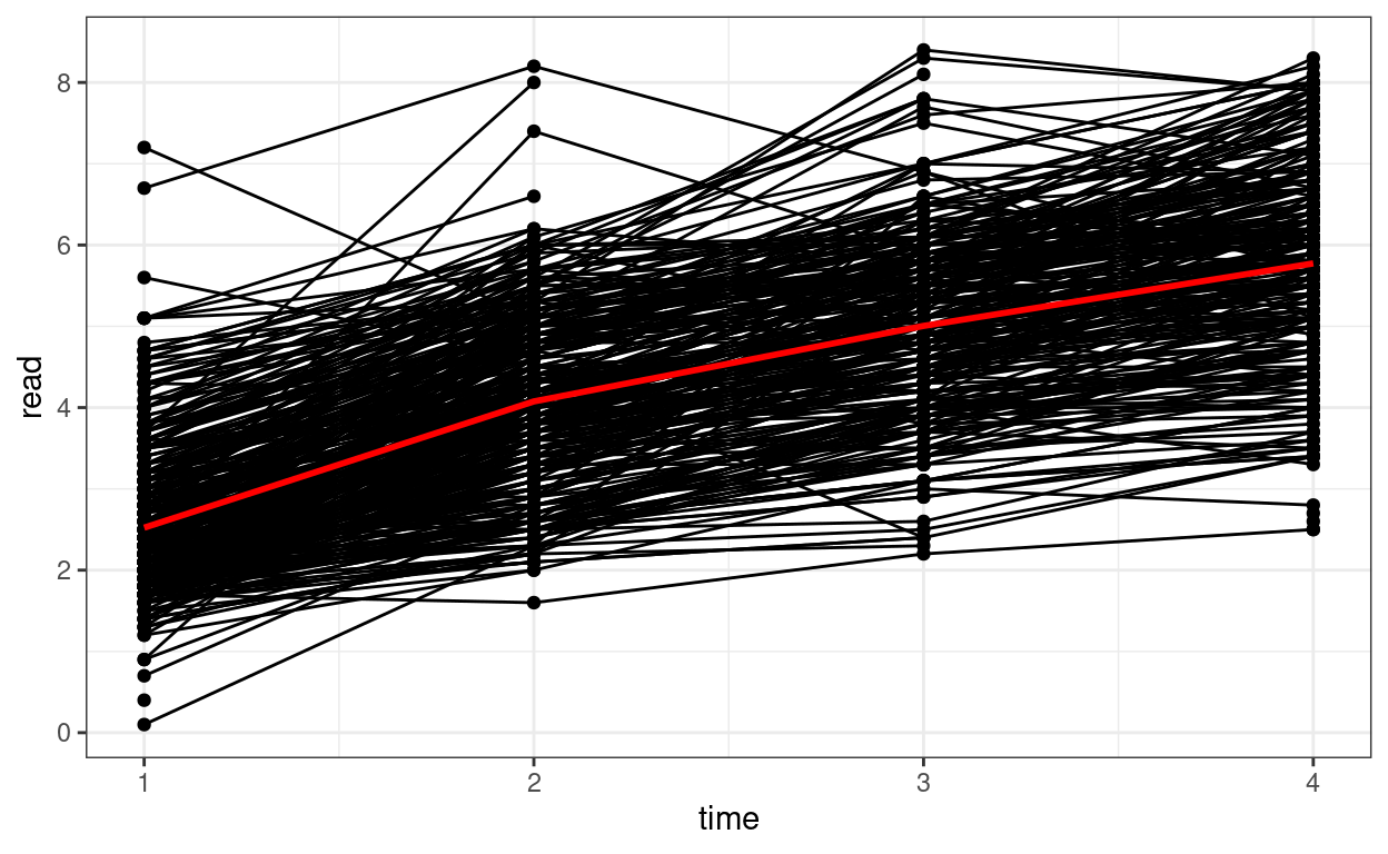
We can see that on average there is an increasing trend across time, but also there is a lot of variations in each individual’s starting point and the trajectory of change.
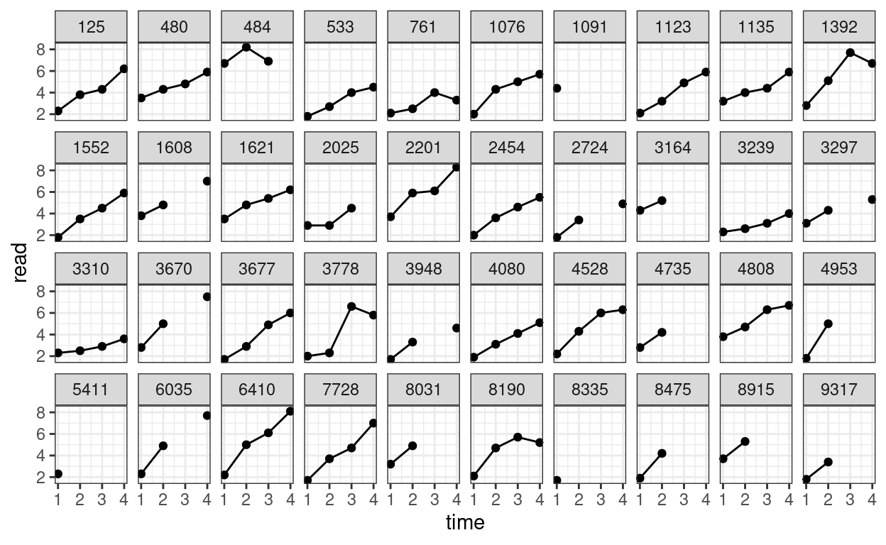
We can also plot the trajectory for a random sample of individuals:
# Randomly sample 40 individuals
set.seed(1349)
sampled_id <- sample(unique(curran_long$id), 40)
curran_long %>%
  filter(id %in% sampled_id) %>%
  ggplot(aes(x = time, y = read)) +
  geom_point() +
  geom_line() +  # add lines to connect the data for each person
  facet_wrap(~ id, ncol = 10)
Temporal Covariances and Correlations
# Easier with the wide data set
# Covariance matrix:
curran_wide %>%
  select(starts_with("read")) %>%
  cov(use = "complete") %>%   # listwise deletion
  round(2L)  # two decimal places
>#       read1 read2 read3 read4
># read1  0.77  0.55  0.52  0.48
># read2  0.55  1.01  0.90  0.92
># read3  0.52  0.90  1.22  1.09
># read4  0.48  0.92  1.09  1.48
# Correlation matrix
curran_wide %>%
select(starts_with("read")) %>%
cor(use = "complete") %>% # listwise deletion
round(2L) # two decimal places
>#       read1 read2 read3 read4
># read1  1.00  0.62  0.53  0.45
># read2  0.62  1.00  0.81  0.75
># read3  0.53  0.81  1.00  0.81
># read4  0.45  0.75  0.81  1.00
You can see the variances increase over time, and the correlation is generally stronger for observations closer in time.
Attrition Analyses
To see whether those who dropped out or had missing data differed in
some characteristics as those who did not drop out, let’s identify the
group with complete data on read, and the group without
complete data on read
# Create grouping
curran_wide <- curran_wide %>%
  # Compute summaries by rows
  rowwise() %>%
  # First compute the number of missing occasions
  mutate(nmis_read = sum(is.na(c_across(read1:read4))),
         # Complete only when nmis_read = 0
         complete = if_else(nmis_read == 0, "complete", "incomplete")) %>%
  ungroup()
# Compare the differences
datasummary((anti1 + read1 + kidgen + momage + kidage + homecog + homeemo) ~
              complete * (Mean + SD), data = curran_wide)
| Mean | SD | Mean | SD | |
|---|---|---|---|---|
| anti1 | 1.49 | 1.54 | 1.89 | 1.78 |
| read1 | 2.50 | 0.88 | 2.55 | 0.99 |
| kidgen | 0.52 | 0.50 | 0.48 | 0.50 |
| momage | 25.61 | 1.85 | 25.42 | 1.92 |
| kidage | 6.90 | 0.62 | 6.97 | 0.66 |
| homecog | 9.09 | 2.46 | 8.63 | 2.70 |
| homeemo | 9.35 | 2.23 | 9.01 | 2.41 |
The two groups are pretty similar, except that the group with missing
seem to have higher baseline antisocial score, and lower
homecog. In actually analyses, you may want to adjust for
these variables by including them in the model (as covariates), if you
suspect the results may be confounded by higher probability of dropping
out.
Of course, the two groups could still be different in important characteristics that are not included in the data. It requires careful investigation of why the data were missing
Unconditional Model
You can use the lme4 package for the basic model:
># Linear mixed model fit by REML. t-tests use Satterthwaite's method [
># lmerModLmerTest]
># Formula: read ~ (1 | id)
>#    Data: curran_long
>#
># REML criterion at convergence: 5056
>#
># Scaled residuals:
>#     Min      1Q  Median      3Q     Max
># -2.2170 -0.7940  0.0235  0.7247  2.3434
>#
># Random effects:
>#  Groups   Name        Variance Std.Dev.
>#  id       (Intercept) 0.30     0.548
>#  Residual             2.39     1.546
># Number of obs: 1325, groups:  id, 405
>#
># Fixed effects:
>#             Estimate Std. Error       df t value Pr(>|t|)
># (Intercept)   4.1128     0.0509 379.7112    80.8   <2e-16 ***
># ---
># Signif. codes:  0 '***' 0.001 '**' 0.01 '*' 0.05 '.' 0.1 ' ' 1
However, lme4 has some limitations with longitudinal
data analysis, as it assumes that what is called a compound symmetry
error covariance structure. Basically that means that the within-person
(level-1) error has constant variance (i.e., \(\sigma^2\)) over time, and the errors from
one time point to the next is not correlated after conditioning on the
fixed and random effects. In other words, whatever that causes one to
has a higher (or lower) score than predicted for today will not carry
over for tomorrow.
There are a few more flexible packages for handling longitudinal
data. You will see people use nlme a lot. There are also
packages with Bayesian estimation, such as MCMCglmm and
brms. For this class, we will use glmmTMB, a
package that has a lot of the features for longitudinal data and has a
very similar structure as lme4. Let’s replicate the results
from lme4:
# Default in glmmTMB is ML; need to specify REML is desired
m00 <- glmmTMB(read ~ (1 | id), data = curran_long, REML = TRUE)
summary(m00)
>#  Family: gaussian  ( identity )
># Formula:          read ~ (1 | id)
># Data: curran_long
>#
>#      AIC      BIC   logLik deviance df.resid
>#     5062     5078    -2528     5056     1323
>#
># Random effects:
>#
># Conditional model:
>#  Groups   Name        Variance Std.Dev.
>#  id       (Intercept) 0.30     0.548
>#  Residual             2.39     1.546
># Number of obs: 1325, groups:  id, 405
>#
># Dispersion estimate for gaussian family (sigma^2): 2.39
>#
># Conditional model:
>#             Estimate Std. Error z value Pr(>|z|)
># (Intercept)   4.1128     0.0513    80.2   <2e-16 ***
># ---
># Signif. codes:  0 '***' 0.001 '**' 0.01 '*' 0.05 '.' 0.1 ' ' 1
You can see that the results are similar. Let’s look at the ICC (i.e., proportion of variance at the between-person level).
(vc_m00 <- VarCorr(m00)) # shows the random effect SDs
>#
># Conditional model:
>#  Groups   Name        Std.Dev.
>#  id       (Intercept) 0.548
># Residual 1.546vc_m00[[1]]$id[1, 1] # intercept variance (tau_0^2)
># [1] 0.3005attr(vc_m00[[1]], "sc")^2 # lv-1 error variance (sigma^2)
># [1] 2.39# ICC: tau_0^2 / (tau_0^2 + sigma^2)
vc_m00[[1]]$id[1, 1] /
(vc_m00[[1]]$id[1, 1] + attr(vc_m00[[1]], "sc")^2)
># [1] 0.1117Unstructured Fixed Part/Compound Symmetry* (15.1.1 of Snijders & Bosker, 2012)
Instead of assuming a specific growth shape (e.g., linear), one can instead just allow each time point to have its own mean. This provides good fit to the data, but is limited because it does not allow for interpretable description of how individuals change over time, and does not test for any trends. Therefore, more commonly it is used as a comparison to more simplified growth models.
# Compound Symmetry (i.e., same as repeated measure ANOVA)
# Use `0 +` to suppress the intercept
m_cs <- glmmTMB(read ~ 0 + factor(time) + (1 | id),
  data = curran_long,
  REML = TRUE
)
summary(m_cs)  # omnibus test for time
>#  Family: gaussian  ( identity )
># Formula:          read ~ 0 + factor(time) + (1 | id)
># Data: curran_long
>#
>#      AIC      BIC   logLik deviance df.resid
>#     3388     3419    -1688     3376     1323
>#
># Random effects:
>#
># Conditional model:
>#  Groups   Name        Variance Std.Dev.
>#  id       (Intercept) 0.790    0.889
>#  Residual             0.407    0.638
># Number of obs: 1325, groups:  id, 405
>#
># Dispersion estimate for gaussian family (sigma^2): 0.407
>#
># Conditional model:
>#               Estimate Std. Error z value Pr(>|z|)
># factor(time)1   2.5227     0.0544    46.4   <2e-16 ***
># factor(time)2   4.0680     0.0555    73.3   <2e-16 ***
># factor(time)3   5.0119     0.0601    83.3   <2e-16 ***
># factor(time)4   5.8122     0.0604    96.2   <2e-16 ***
># ---
># Signif. codes: 0 '***' 0.001 '**' 0.01 '*' 0.05 '.' 0.1 ' ' 1From this model you can compute the conditional ICC, which is the proportion of between-person variance out of the total variance in the detrended data.
(vc_cs <- VarCorr(m_cs)) # shows the random effect SDs
>#
># Conditional model:
>#  Groups   Name        Std.Dev.
>#  id       (Intercept) 0.889
># Residual 0.638vc_cs[[1]]$id[1, 1] # intercept variance (tau_0^2)
># [1] 0.79attr(vc_cs[[1]], "sc")^2 # lv-1 error variance (sigma^2)
># [1] 0.4075# ICC: tau_0^2 / (tau_0^2 + sigma^2)
vc_cs[[1]]$id[1, 1] /
(vc_cs[[1]]$id[1, 1] + attr(vc_cs[[1]], "sc")^2)
># [1] 0.6597So after removing the trend, the between-person variance is larger than the within-person variance.
Linear Growth Models
Linear Model With Time
Level 1: Within-Person
\[\text{read}_{ti} = \beta_{0i} + \beta_{1i} \text{time}_{ti} + e_{ti}\]
Level 2: Between-Person
\[ \begin{aligned} \beta_{0i} = \gamma_{00} + u_{0i} \\ \beta_{1i} = \gamma_{10} + u_{1i} \end{aligned} \]
# Make 0 the initial time
curran_long <- curran_long %>%
  mutate(time0 = time - 1)
# Fit a linear growth model with no random slopes (not commonly done)
m_gca <- glmmTMB(read ~ time0 + (time0 | id), data = curran_long, REML = TRUE)
summary(m_gca)
># Family: gaussian ( identity )
># Formula: read ~ time0 + (time0 | id)
># Data: curran_long
>#
># AIC BIC logLik deviance df.resid
># 3394 3425 -1691 3382 1321
>#
># Random effects:
>#
># Conditional model:
># Groups Name Variance Std.Dev. Corr
># id (Intercept) 0.5731 0.757
># time0 0.0746 0.273 0.29
># Residual 0.3458 0.588
># Number of obs: 1325, groups: id, 405
>#
># Dispersion estimate for gaussian family (sigma^2): 0.346
>#
># Conditional model:
># Estimate Std. Error z value Pr(>|z|)
># (Intercept) 2.6961 0.0453 59.5 <2e-16 ***
># time0 1.1191 0.0218 51.3 <2e-16 ***
># ---
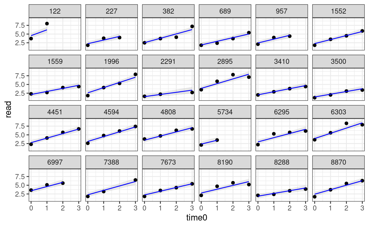
># Signif. codes: 0 '***' 0.001 '**' 0.01 '*' 0.05 '.' 0.1 ' ' 1random_persons <- sample(unique(curran_long$id), size = 24)
broom.mixed::augment(m_gca) %>%
# Select only the 24 participants
filter(id %in% random_persons) %>%
ggplot(aes(x = time0, y = read)) +
geom_point() +
# Add 95% confidence band
geom_ribbon(aes(ymin = .fitted - 2 * .se.fit,
ymax = .fitted + 2 * .se.fit),
alpha = 0.1) +
geom_line(aes(y = .fitted), col = "blue") +
facet_wrap(~ id, ncol = 6)
Piecewise Growth Model
A piecewise linear growth assumes that there are two or more phases of linear change across time. For example, we can assume that, for our data, phase 1 is from Time 0 to Time 1, and phase 2 is from Time 1 to Time 3.
Because we’re estimating two slopes, we need two predictors:
phase1 represents the initial slope from Time 0 to Time 1,
and phase2 represents the slope from Time 1 to Time 3. The
coding is shown below:
\[\begin{bmatrix} \textrm{phase1} & \textrm{phase2} \\ 0 & 0 \\ 1 & 0 \\ 1 & 1 \\ 1 & 2 \end{bmatrix}\]
To understand the coding, in phase1 the line changes
from Time 0 to Time 1, but stays there. phase2 has 0 from
Time 0 to Time 1 as nothing should have happened. Then, From Time 1 to
Time 3 it starts to increase linearly.
One way to check whether you’ve specified the coding correctly is to sum the numbers in every row, which you should get back 0, 1, 2, 3, . . .
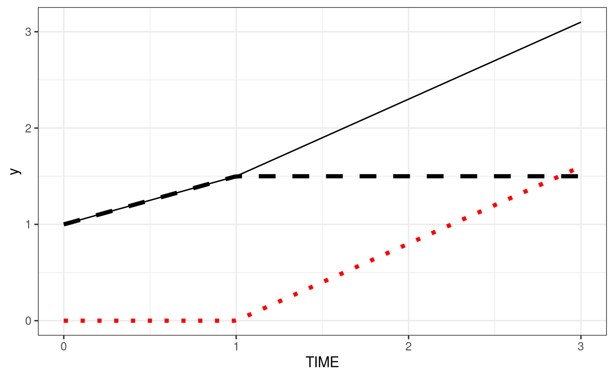
Below is an example where intercept = 1, growth in phase 1 = 0.5, growth in phase 2 = 0.8. The dashed line shows the contribution from phase1 (plus the intercept). The red dotted line shows the contribution from phase2.
demo_df <- tibble(TIME = c(0, 1, 2, 3))
ggplot(demo_df, aes(x = TIME)) +
  stat_function(fun = function(x) 1 + 0.5 * pmin(x, 1),
                linetype = "dashed", size = 1.5) +
  stat_function(fun = function(x) 0.8 * pmax(x - 1, 0), col = "red",
                linetype = "dotted", size = 1.5) +
  stat_function(fun = function(x) 1 + 0.5 * pmin(x, 1) + 0.8 * pmax(x - 1, 0))
Now, we assume Time 0 to Time 1 has one slope, and Time 1 to Time 3 has another slope.
# Compute phase1 and phase2
curran_long <- curran_long %>%
  mutate(phase1 = pmin(time0, 1),  # anything bigger than 1 becomes 1
         phase2 = pmax(time0 - 1, 0))  # set time to start at TIME 1, and then make
# anything smaller than 0 to 0
# Check the coding:
curran_long %>%
  select(time0, phase1, phase2) %>%
  distinct()
># # A tibble: 4 × 3
>#   time0 phase1 phase2
>#   <dbl>  <dbl>  <dbl>
># 1     0      0      0
># 2     1      1      0
># 3     2      1      1
># 4     3      1      2
# Fit the piecewise growth model
m_pw <- glmmTMB(read ~ phase1 + phase2 + (phase1 + phase2 | id),
data = curran_long, REML = TRUE,
# The default optimizer did not converge; try optim
control = glmmTMBControl(
optimizer = optim,
optArgs = list(method = "BFGS")
)
)
summary(m_pw)
>#  Family: gaussian  ( identity )
># Formula:          read ~ phase1 + phase2 + (phase1 + phase2 | id)
># Data: curran_long
>#
>#      AIC      BIC   logLik deviance df.resid
>#     3230     3282    -1605     3210     1318
>#
># Random effects:
>#
># Conditional model:
>#  Groups   Name        Variance Std.Dev. Corr
>#  id       (Intercept) 0.6052   0.778
>#           phase1      0.2270   0.476     0.13
>#           phase2      0.0536   0.232    -0.15  0.96
>#  Residual             0.2514   0.501
># Number of obs: 1325, groups:  id, 405
>#
># Dispersion estimate for gaussian family (sigma^2): 0.251
>#
># Conditional model:
>#             Estimate Std. Error z value Pr(>|z|)
># (Intercept)   2.5227     0.0460    54.9   <2e-16 ***
># phase1        1.5621     0.0427    36.6   <2e-16 ***
># phase2        0.8793     0.0255    34.5   <2e-16 ***
># ---
># Signif. codes:  0 '***' 0.001 '**' 0.01 '*' 0.05 '.' 0.1 ' ' 1
Plotting the predicted trajectories
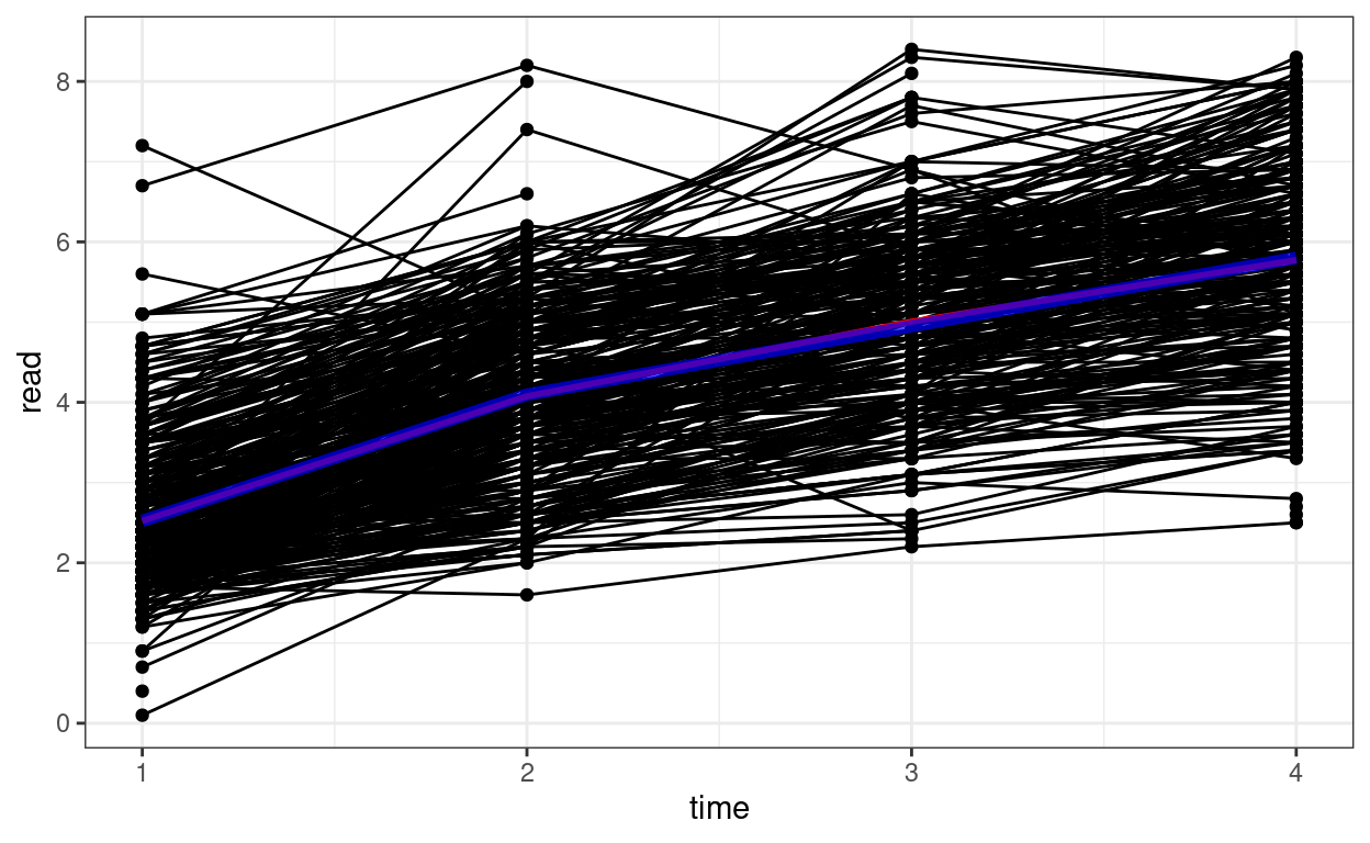
Average predicted trajectory on the spaghetti plot:
# Plot the predicted growth shape (in blue):
# `tibble()` is used to create a tibble object, which is the data frame used in
# tidyverse
pred_pw <- tibble(time = 1:4,
                  phase1 = c(0, 1, 1, 1),
                  phase2 = c(0, 0, 1, 2),
                  id = NA)
pred_pw <- pred_pw %>%
  mutate(read = predict(m_pw, newdata = pred_pw, re.form = NA))
p1 +
  geom_line(data = pred_pw, col = "blue", size = 2, alpha = 0.7)
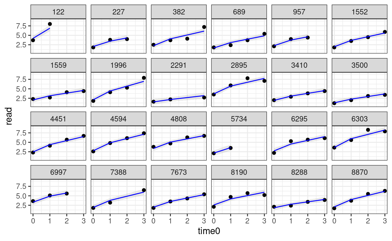
Predicted trajectories at the individual level
# Add predicted lines to individual trajectories
broom.mixed::augment(m_pw) %>%
  # compute the original time
  mutate(time0 = phase1 + phase2) %>%
  # Select only the 24 participants
  filter(id %in% random_persons) %>%
  ggplot(aes(x = time0, y = read)) +
  geom_point() +
  # Add 95% confidence band
  geom_ribbon(aes(ymin = .fitted - 2 * .se.fit,
                  ymax = .fitted + 2 * .se.fit),
              alpha = 0.1) +
  geom_line(aes(y = .fitted), col = "blue") +
  facet_wrap(~ id, ncol = 6)
Saturated Model* (15.1.3 of Snijders & Bosker, 2012)
This is what is called the fully multivariate model in the text. The model is saturated in the sense that it perfectly fits the means and covariances of the outcome variable among the various time points. The model, however, does not allow one to test any structure one is interested, so in practice it is mostly used to check how good or bad the chosen model deviates from this “perfect” model.
# I use ML estimation so that both the fixed and the random part can be compared
m_sat_ml <- glmmTMB(read ~ 0 + factor(time) + (0 + factor(time) | id),
  dispformula = ~0,
  data = curran_long
)
m_gca_ml <- glmmTMB(read ~ time0 + (time0 | id), data = curran_long)
m_pw_ml <- glmmTMB(read ~ phase1 + phase2 + (phase1 + phase2 | id),
  data = curran_long,
  # The default optimizer did not converge; try optim
  control = glmmTMBControl(
    optimizer = optim,
    optArgs = list(method = "BFGS")
  )
)
# Compare the models
anova(m_sat_ml, m_gca_ml, m_pw_ml)
># Data: curran_long
># Models:
># m_gca_ml: read ~ time0 + (time0 | id), zi=~0, disp=~1
># m_pw_ml: read ~ phase1 + phase2 + (phase1 + phase2 | id), zi=~0, disp=~1
># m_sat_ml: read ~ 0 + factor(time) + (0 + factor(time) | id), zi=~0, disp=~0
>#          Df  AIC  BIC logLik deviance  Chisq Chi Df Pr(>Chisq)
># m_gca_ml  6 3384 3415  -1686     3372
># m_pw_ml  10 3215 3267  -1598     3195 176.41      4     <2e-16 ***
># m_sat_ml 14 3218 3291  -1595     3190   5.32      4       0.26
># ---
># Signif. codes:  0 '***' 0.001 '**' 0.01 '*' 0.05 '.' 0.1 ' ' 1
The above shows that the fit of the piecewise model was not significantly worse than the saturated model.
Time-Invariant Covariates
Time-invariant covariate = Another way to say a level-2 variable
You can add homecog and its interaction to the model
with age as predictor. Just that now there are two interaction terms:
one with the first piece and the other with the second piece.
# Add `homecog` and its interaction with growth
# First, center homecog to 9
curran_long$homecog9 <- curran_long$homecog - 9
m_pw_homecog <- glmmTMB(
  read ~ (phase1 + phase2) * homecog9 +
    (phase1 + phase2 | id),
  data = curran_long,
  REML = TRUE,
  # The default optimizer did not converge; try optim
  control = glmmTMBControl(
    optimizer = optim,
    optArgs = list(method = "BFGS")
  )
)
summary(m_pw_homecog)
># Family: gaussian ( identity )
># Formula:
># read ~ (phase1 + phase2) * homecog9 + (phase1 + phase2 | id)
># Data: curran_long
>#
># AIC BIC logLik deviance df.resid
># 3237 3304 -1605 3211 1318
>#
># Random effects:
>#
># Conditional model:
># Groups Name Variance Std.Dev. Corr
># id (Intercept) 0.594 0.771
># phase1 0.215 0.464 0.10
># phase2 0.053 0.230 -0.17 0.96
># Residual 0.252 0.502
># Number of obs: 1325, groups: id, 405
>#
># Dispersion estimate for gaussian family (sigma^2): 0.252
>#
># Conditional model:
># Estimate Std. Error z value Pr(>|z|)
># (Intercept) 2.5273 0.0457 55.2 <2e-16 ***
># phase1 1.5667 0.0424 37.0 <2e-16 ***
># phase2 0.8798 0.0255 34.6 <2e-16 ***
># homecog9 0.0436 0.0178 2.5 0.014 *
># phase1:homecog9 0.0415 0.0166 2.5 0.012 *
># phase2:homecog9 0.0105 0.0101 1.0 0.296
># ---
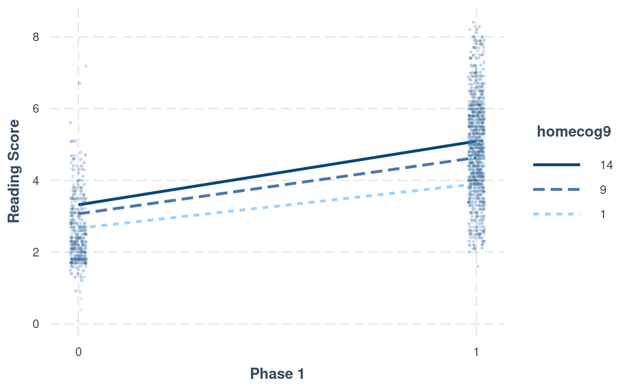
># Signif. codes: 0 '***' 0.001 '**' 0.01 '*' 0.05 '.' 0.1 ' ' 1# Interaction plot (phase1:homecog)
interact_plot(m_pw_homecog,
pred = "phase1",
modx = "homecog9",
modx.values = c(1, 9, 14) - 9,
modx.labels = c(1, 9, 14),
plot.points = TRUE,
point.size = 0.5,
point.alpha = 0.2,
jitter = 0.02,
x.label = "Phase 1",
y.label = "Reading Score")
# Interaction plot (phase2:homecog)
interact_plot(m_pw_homecog,
              pred = "phase2",
              modx = "homecog9",
              modx.values = c(1, 9, 14) - 9,
              modx.labels = c(1, 9, 14),
              plot.points = TRUE,
              point.size = 0.5,
              point.alpha = 0.2,
              jitter = 0.02,
              x.label = "Phase 2",
              y.label = "Reading Score")
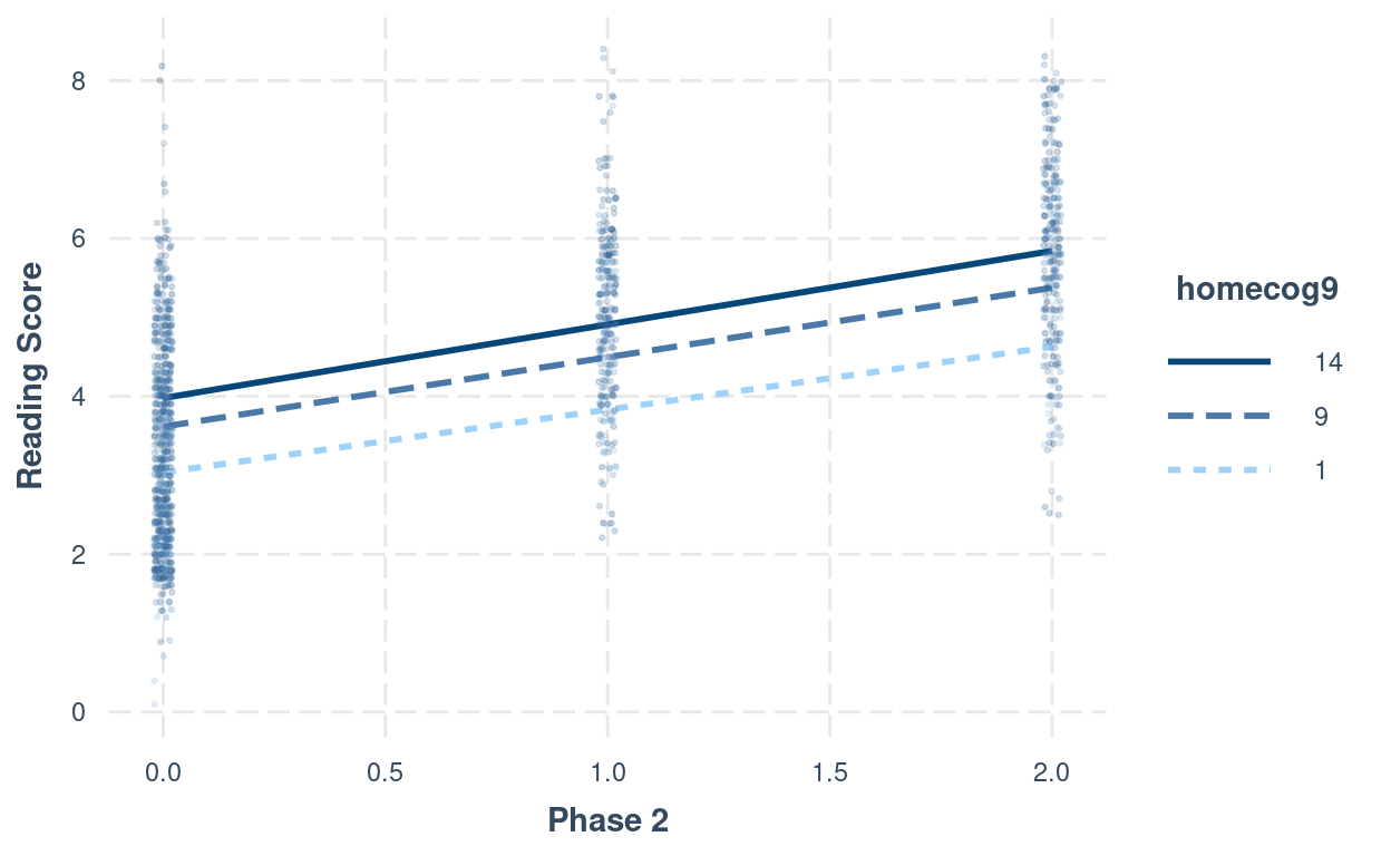
Table of Coefficients
msummary(
  list(
    "Compound Symmetry" = m00,
    "GCA" = m_gca,
    "Piecewise" = m_pw,
    "Piecewise + homecog" = m_pw_homecog
  ),
  group = group + term ~ model
)
| Compound Symmetry | GCA | Piecewise | Piecewise + homecog | ||
|---|---|---|---|---|---|
| (Intercept) | 4.113 | 2.696 | 2.523 | 2.527 | |
| (0.051) | (0.045) | (0.046) | (0.046) | ||
| time0 | 1.119 | ||||
| (0.022) | |||||
| phase1 | 1.562 | 1.567 | |||
| (0.043) | (0.042) | ||||
| phase2 | 0.879 | 0.880 | |||
| (0.025) | (0.025) | ||||
| homecog9 | 0.044 | ||||
| (0.018) | |||||
| phase1 × homecog9 | 0.042 | ||||
| (0.017) | |||||
| phase2 × homecog9 | 0.011 | ||||
| (0.010) | |||||
| id | sd__(Intercept) | 0.548 | 0.757 | 0.778 | 0.771 |
| sd__time0 | 0.273 | ||||
| cor__(Intercept).time0 | 0.286 | ||||
| sd__phase1 | 0.476 | 0.464 | |||
| sd__phase2 | 0.232 | 0.230 | |||
| cor__(Intercept).phase1 | 0.129 | 0.104 | |||
| cor__(Intercept).phase2 | −0.154 | −0.168 | |||
| cor__phase1.phase2 | 0.957 | 0.961 | |||
| Residual | sd__Observation | 1.546 | 0.588 | 0.501 | 0.502 |
| Num.Obs. | 1325 | 1325 | 1325 | 1325 | |
| AIC | 5061.9 | 3394.0 | 3229.7 | 3236.7 | |
| BIC | 5077.5 | 3425.1 | 3281.6 | 3304.1 | |
| Log.Lik. | −2527.974 | −1691.000 | −1604.869 | −1605.341 |
Variable Occasions
MLM can handle varying measurement occasions. For example, maybe some students are first measured in September when the semester starts, whereas other students are first measured in October or November. How important this difference depends on the research being studied. For especially infant/early childhood research, one month can already mean a lot of growth, and so it is important to take that into account.
Instead of using time, one can instead model an outcome
variable as a function of age, with the kidage variable. To
use age, however, one may not want to start at age = 0. In the data set,
the minimum age is 6. Therefore, we can subtract 6 from the
original kidage variable, so that the zero point represent
someone at age = 6.
Quadratic Function
Here is an example:
# Subtract age by 6
curran_long <- curran_long %>%
mutate(kidagetv = kidage + time * 2,
# Compute the age for each time point
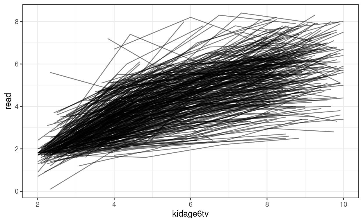
kidage6tv = kidagetv - 6)
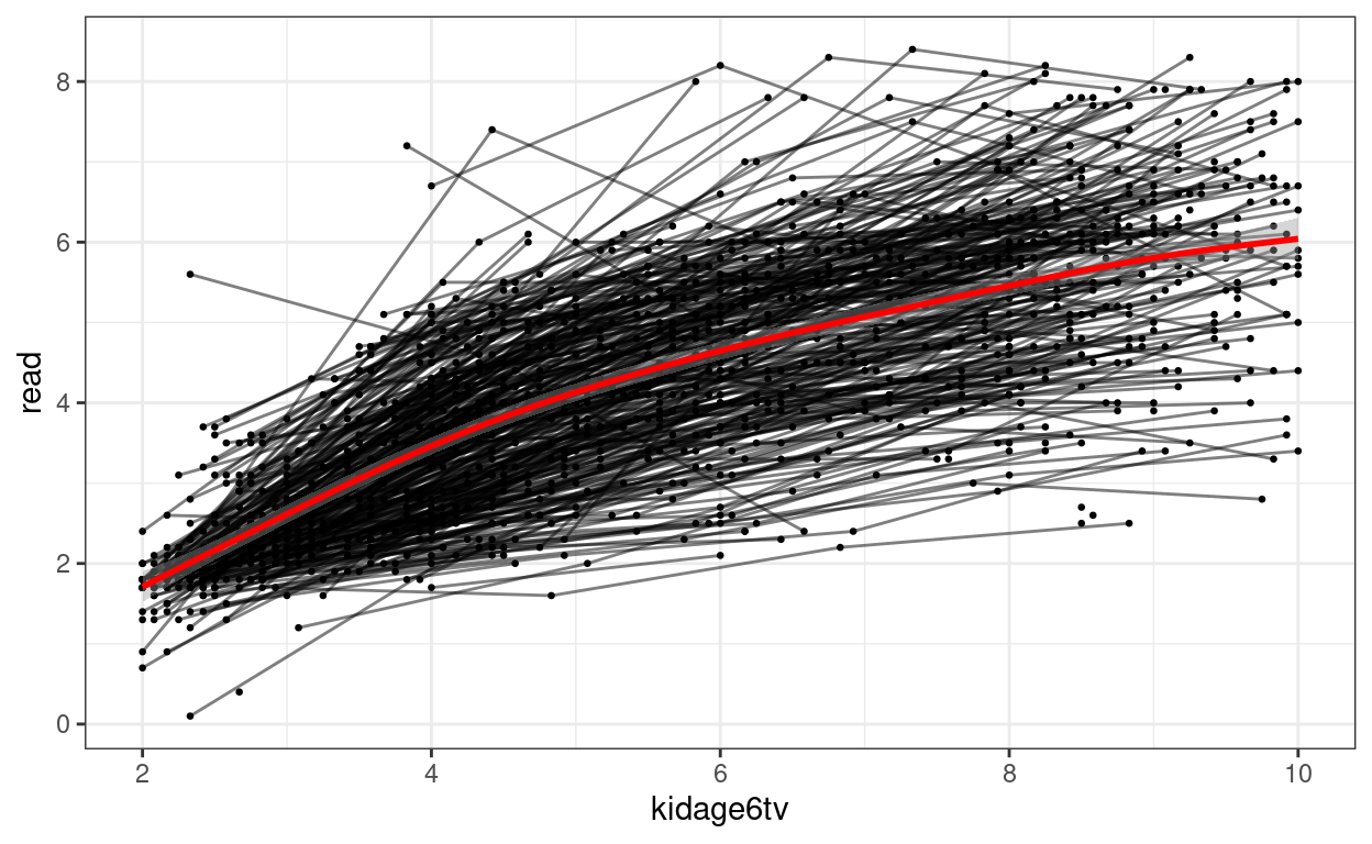
# Plot the data
ggplot(curran_long, aes(x = kidage6tv, y = read)) +
geom_point(size = 0.5) +
# add lines to connect the data for each person
geom_line(aes(group = id), alpha = 0.5) +
# add a mean trajectory
geom_smooth(col = "red", size = 1)
# Fit a quadratic model
m_agesq <- glmmTMB(
  read ~ kidage6tv + I(kidage6tv^2) +
    (kidage6tv + I(kidage6tv^2) | id),
  data = curran_long,
  REML = TRUE
)
summary(m_agesq)
># Family: gaussian ( identity )
># Formula:
># read ~ kidage6tv + I(kidage6tv^2) + (kidage6tv + I(kidage6tv^2) |
># id)
># Data: curran_long
>#
># AIC BIC logLik deviance df.resid
># 3006 3058 -1493 2986 1318
>#
># Random effects:
>#
># Conditional model:
># Groups Name Variance Std.Dev. Corr
># id (Intercept) 0.29419 0.5424
># kidage6tv 0.19048 0.4364 -0.98
># I(kidage6tv^2) 0.00093 0.0305 0.90 -0.96
># Residual 0.24615 0.4961
># Number of obs: 1325, groups: id, 405
>#
># Dispersion estimate for gaussian family (sigma^2): 0.246
>#
># Conditional model:
># Estimate Std. Error z value Pr(>|z|)
># (Intercept) -0.32074 0.09683 -3.31 0.00093 ***
># kidage6tv 1.12846 0.04219 26.75 < 2e-16 ***
># I(kidage6tv^2) -0.04958 0.00348 -14.24 < 2e-16 ***
># ---
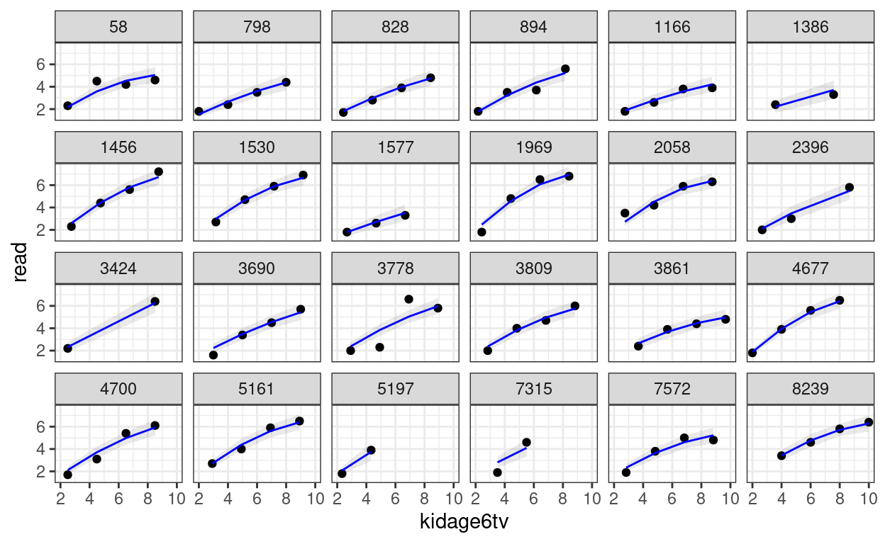
># Signif. codes: 0 '***' 0.001 '**' 0.01 '*' 0.05 '.' 0.1 ' ' 1You can then perform the diagnostics and see whether the individual growth shape appears to be quadratic.
random_persons <- sample(unique(curran_long$id), size = 24)
broom.mixed::augment(m_agesq) %>%
  # Select only the 24 participants
  filter(id %in% random_persons) %>%
  ggplot(aes(x = kidage6tv, y = read)) +
  geom_point() +
  # Add 95% confidence band
  geom_ribbon(aes(ymin = .fitted - 2 * .se.fit,
                  ymax = .fitted + 2 * .se.fit),
              alpha = 0.1) +
  geom_line(aes(y = .fitted), col = "blue") +
  facet_wrap(~ id, ncol = 6)
# Plot the predicted trajectories on the same panel
broom.mixed::augment(m_agesq) %>%
  ggplot(aes(x = kidage6tv, y = read, group = factor(id))) +
  geom_line(alpha = 0.5)