\[ \newcommand{\bv}[1]{\boldsymbol{\mathbf{#1}}} \]
Click here to download the Rmd file: week7-mlm-exp.Rmd
Load Packages and Import Data
# To install a package, run the following ONCE (and only once on your computer)
# install.packages("psych")
library(here)  # makes reading data more consistent
library(tidyverse)  # for data manipulation and plotting
library(haven)  # for importing SPSS/SAS/Stata data
library(lme4)  # for multilevel analysis
library(lmerTest)  # for testing coefficients
library(MuMIn)  # for R^2
library(sjPlot)  # for plotting effects
library(emmeans)  # for marginal means
library(modelsummary)  # for making tables
theme_set(theme_bw())  # Theme; just my personal preference
This note focused mostly on within-subjects experimental designs, as between-subjects designs are generally easier to handle with the treatment condition at the upper level. When clusters of people are randomly assigned, the design is called a cluster-randomized trial. See an example here: https://www.sciencedirect.com/science/article/abs/pii/S0022103117300860
# Data example of Hoffman & Atchley (2001)
# Download from the Internet, unzip, and read in
zip_path <- here("data_files", "MLM_for_Exp_Appendices.zip")
if (!file.exists(zip_path)) {
    download.file(
        "http://www.lesahoffman.com/Research/MLM_for_Exp_Appendices.zip",
        zip_path
    )
}
driving_dat <- read_sav(unz(zip_path, "MLM_for_Exp_Appendices/Ex1.sav"))
# Convert `sex` and `oldage` to factor
# Note: also convert id and Item to factor (just for plotting)
driving_dat <- driving_dat %>%
    mutate(
        sex = as_factor(sex),
        oldage = factor(oldage,
            levels = c(0, 1),
            labels = c("Below Age 40", "Over Age 40")
        ),
        # id = factor(id),
        Item = factor(Item)
    )
# Show data
rmarkdown::paged_table(driving_dat)
With SPSS data, you can view the variable labels by
>#          [,1]
># id       "Participant ID"
># sex      "Participant Sex (0=men, 1=women)"
># age      "Age"
># NAME     NULL
># rt_sec   "Response Time in Seconds"
># Item     NULL
># meaning  "Meaning Rating (0-5)"
># salience "Salience Rating (0-5)"
># lg_rt    "Natural Log RT in Seconds"
># oldage   NULL
># older    "Copy of oldage to be treated as categorical"
># yrs65    "Years Over Age 65 (0=65)"
># c_mean   "Centered Meaning (0=3)"
># c_sal    "Centered Salience (0=3)"
Wide and Long Format
The data we used here is in what is called a long format, where each row corresponds to a unique observation, and is required for MLM. More commonly, however, you may have data in a wide format, where each row records multiple observations for each person, as shown below
# Show data
rmarkdown::paged_table(driving_wide)
As can be seen above, rt_sec1 to rt_sec80
are the responses to the 51 items. If you have like the above, you need
to convert it to a long format. In R, this can be achieved using the
pivot_long() function, as part of tidyverse
(in the tidyr package):
driving_wide %>%
    pivot_longer(
        cols = rt_sec1:rt_sec80, # specify the columns of repeated measures
        names_to = "Item", # name of the new column to create to indicate item id
        names_prefix = "rt_sec", # remove "rt_sec" from the item ID column
        values_to = "rt_sec", # name of new column containing the response
    ) %>%
    rmarkdown::paged_table()
Descriptive Statistics
Missing Data Rate for Response Time:
driving_dat %>%
    group_by(id) %>%
    summarise(n_missing = sum(is.na(rt_sec))) %>%
    ggplot(aes(x = n_missing)) +
    geom_bar()
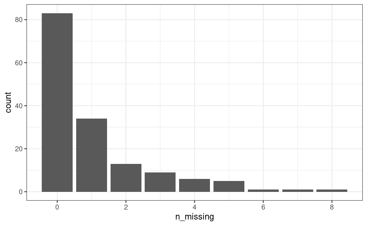
Note that only about 80 people have no missing data
Plotting
Let’s explore the data a bit with
psych::pairs.panels()
driving_dat %>%
    # Select six variables
    select(sex, age, rt_sec, meaning, salience, lg_rt) %>%
    psych::pairs.panels(ellipses = FALSE, cex = 0.2, cex.cor = 1)
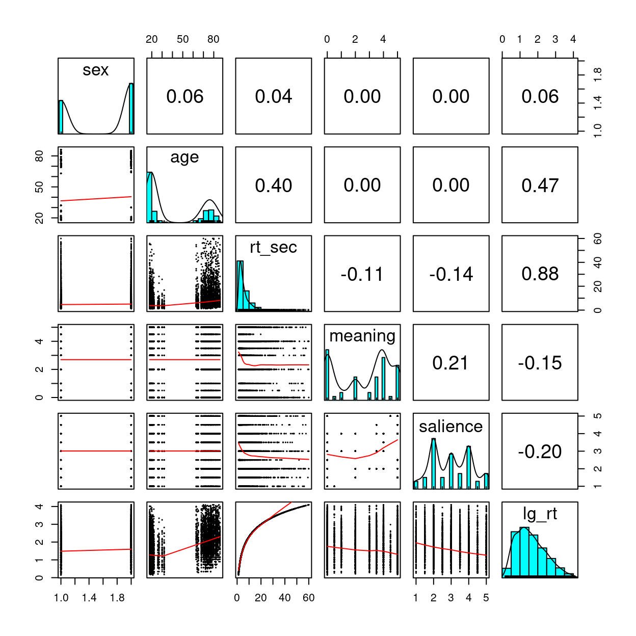
Note the nonnormality in response time. There doesn’t appear to be much gender differences.
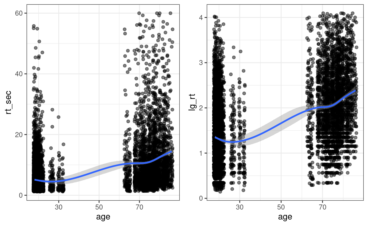
Below is a plot between response time against age:
Left: original response time; Right: Natural log transformation
p1 <- driving_dat %>%
    ggplot(aes(x = age, y = rt_sec)) +
    geom_jitter(width = 0.5, height = 0, alpha = 0.5) +
    geom_smooth()
p2 <- driving_dat %>%
    ggplot(aes(x = age, y = lg_rt)) +
    geom_jitter(width = 0.5, height = 0, alpha = 0.5) +
    geom_smooth()
gridExtra::grid.arrange(p1, p2, ncol = 2)
Cross-Classified Random Effect Analysis
Intraclass Correlations and Design Effects
Note: in the slides I used
lg_rtas the outcome variable, whereas here I directly specify theloginsidelmer(). The two should give identical model fit and estimates. Usinglog(rt_sec)has the benefits that we can get plots on the original response time variable; however, if you prefer plots on the log scale, you may want to uselg_rtinstead.
m0 <- lmer(log(rt_sec) ~ (1 | id) + (1 | Item), data = driving_dat)
vc_m0 <- as.data.frame(VarCorr(m0))
# ICC/Deff (person; cluster size = 51)
icc_person <- vc_m0$vcov[1] / sum(vc_m0$vcov)
# ICC (item; cluster size = 153)
icc_item <- vc_m0$vcov[2] / sum(vc_m0$vcov)
# ICC (person + item)
c("ICC(person + item)" = sum(vc_m0$vcov[1:2]) / sum(vc_m0$vcov))
># ICC(person + item)
>#             0.4399
# For deff(person), need to take out the part for item
c("ICC(person)" = icc_person,
"Deff(person)" = (1 - icc_item) + (51 - 1) * icc_person)
>#  ICC(person) Deff(person)
>#        0.259       13.768
# For deff(item), need to take out the part for person
c("ICC(item)" = icc_item,
"Deff(item)" = (1 - icc_person) + (153 - 1) * icc_item)
>#  ICC(item) Deff(item)
>#     0.1809    28.2386
So both the item and the person levels are needed
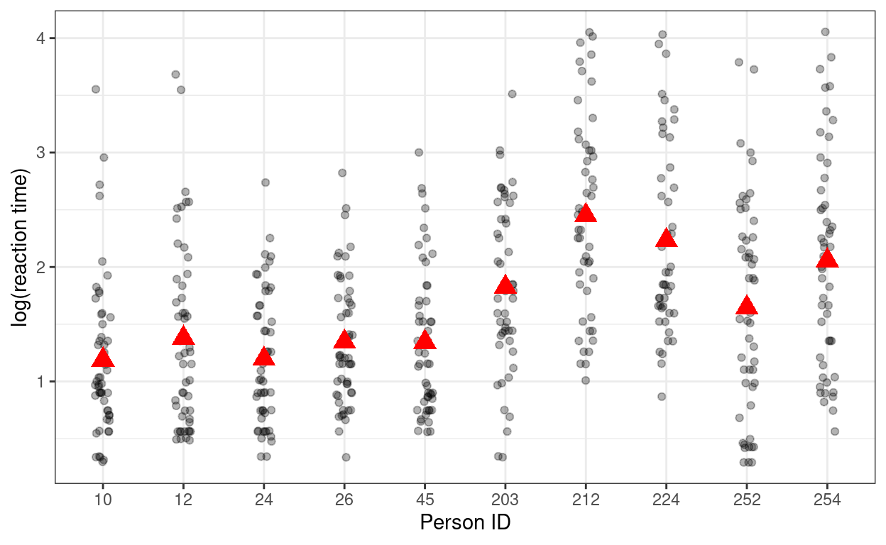
Visualizing person-level and item-level variances
set.seed(2124)
# Variation across persons
random_ids <- sample(unique(driving_dat$id), size = 10)
driving_dat %>%
    filter(id %in% random_ids) %>%  # select only 10 persons
    ggplot(aes(x = factor(id), y = lg_rt)) +
    geom_jitter(height = 0, width = 0.1, alpha = 0.3) +
    # Add person means
    stat_summary(
      fun = "mean",
      geom = "point",
      col = "red",
      shape = 17,  # use triangles
      size = 4  # make them larger
    ) +
    # change axis labels
    labs(x = "Person ID", y = "log(reaction time)")
# Variation across items
random_items <- sample(unique(driving_dat$Item), size = 10)
driving_dat %>%
    filter(Item %in% random_items) %>%  # select only 10 persons
    ggplot(aes(x = factor(Item), y = lg_rt)) +
    geom_jitter(height = 0, width = 0.1, alpha = 0.3) +
    # Add person means
    stat_summary(
      fun = "mean",
      geom = "point",
      col = "red",
      shape = 17,  # use triangles
      size = 4  # make them larger
    ) +
    # change axis labels
    labs(x = "Item ID", y = "log(reaction time)")
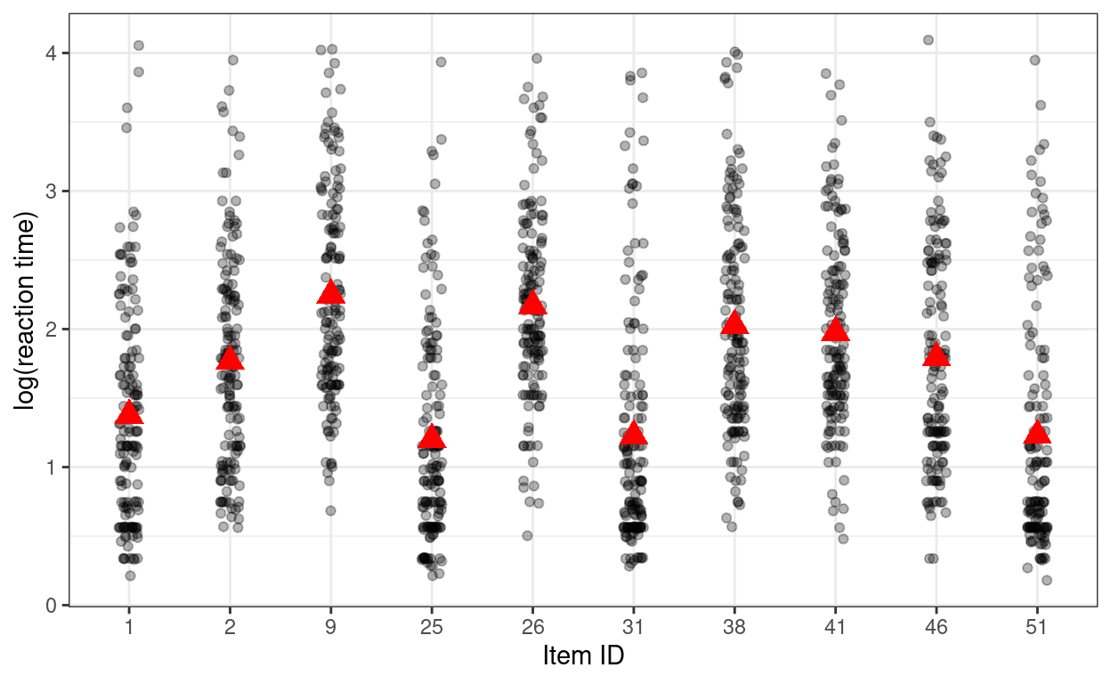
Account for shared variance of item:
- Now, it can be seen that
c_meanandc_salare item-level variables. The model is complex, but one thing that we don’t need to worry is that if the experimental design is balanced (i.e., every item was administered to every person), we don’t need to worry about cluster-means and cluster-mean centering. In this case,c_meanandc_salare purely item-level variables with no person-level variance. You can verify this:
lmer(c_mean ~ (1 | id), data = driving_dat)
># Linear mixed model fit by REML ['lmerModLmerTest']
># Formula: c_mean ~ (1 | id)
>#    Data: driving_dat
># REML criterion at convergence: 32061
># Random effects:
>#  Groups   Name        Std.Dev.
>#  id       (Intercept) 0.00
>#  Residual             1.89
># Number of obs: 7803, groups:  id, 153
># Fixed Effects:
># (Intercept)
>#      -0.353
># optimizer (nloptwrap) convergence code: 0 (OK) ; 0 optimizer warnings; 1 lme4 warnings
You can see that the between-person variance for c_mean
is zero. This, however, does not apply to unbalanced data, in which case
cluster-means will still be needed.
Full Model
Equations
Repeated-Measure level (Lv 1): \[\log(\text{rt_sec}_{i(j,k)}) = \beta_{0(j, k)} + e_{ijk}\] Between-cell (Person \(\times\) Item) level (Lv 2): \[\beta_{0(j, k)} = \gamma_{00} + \beta_{1j} \text{meaning}_{k} + \beta_{2j} \text{salience}_{k} + \beta_{3j} \text{meaning}_{k} \times \text{salience}_{k} + \beta_{4k} \text{oldage}_{j} + u_{0j} + v_{0k}\] Person level (Lv 2a) random slopes \[ \begin{aligned} \beta_{1j} = \gamma_{10} + \gamma_{11} \text{oldage}_{j} + u_{1j} \\ \beta_{2j} = \gamma_{20} + \gamma_{21} \text{oldage}_{j} + u_{2j} \\ \beta_{3j} = \gamma_{30} + \gamma_{31} \text{oldage}_{j} + u_{3j} \\ \end{aligned} \] Item level (Lv2b) random slopes \[\beta_{4k} = \gamma_{40} + v_{4k}\] Combined equations \[ \begin{aligned} \log(\text{rt_sec}_{i(j,k)}) & = \gamma_{00} \\ & + \gamma_{10} \text{meaning}_{k} + \gamma_{20} \text{salience}_{k} + \gamma_{30} \text{meaning}_{k} \times \text{salience}_{k} + \gamma_{40} \text{oldage}_{j} \\ & + \gamma_{11} \text{meaning}_{k} \times \text{oldage}_{j} + \gamma_{21} \text{salience}_{k} \times \text{oldage}_{j} + \gamma_{31} \text{meaning}_{k} \times \text{oldage}_{j} \times \text{oldage}_{j} + \\ & + u_{0j} + u_{1j} \text{meaning}_{k} + u_{2j} \text{salience}_{k} + u_{3j} \text{meaning}_{k} \times \text{salience}_{k} \\ & + v_{0k} + v_{4k} \text{oldage}_{j} \\ & + e_{ijk} \end{aligned} \]
Testing random slopes
The random slopes can be tested one by one
# First, no random slopes
m1 <- lmer(log(rt_sec) ~ c_mean * c_sal * oldage + (1 | id) + (1 | Item),
           data = driving_dat)
# Then test random slopes one by one
# Random slopes of oldage (person-level) across items
m1_rs1 <- lmer(
    log(rt_sec) ~ c_mean * c_sal * oldage + (1 | id) + (oldage | Item),
    data = driving_dat
)
# Test (see the line that says "oldage in (oldage | Item)")
ranova(m1_rs1)  # statistically significant, indicating varying slopes of
># ANOVA-like table for random-effects: Single term deletions
>#
># Model:
># log(rt_sec) ~ c_mean + c_sal + oldage + (1 | id) + (oldage | Item) + c_mean:c_sal + c_mean:oldage + c_sal:oldage + c_mean:c_sal:oldage
>#                           npar logLik   AIC LRT Df Pr(>Chisq)
># <none>                      13  -7401 14829
># (1 | id)                    12  -7552 15127 300  1     <2e-16 ***
># oldage in (oldage | Item)   11  -7457 14936 111  2     <2e-16 ***
># ---
># Signif. codes:  0 '***' 0.001 '**' 0.01 '*' 0.05 '.' 0.1 ' ' 1
# oldage
# Random slopes of c_mean (item-level) across persons
m1_rs2 <- lmer(log(rt_sec) ~ c_mean * c_sal * oldage + (c_mean:c_sal | id) +
(1 | Item),
data = driving_dat)
# Test (see the line that says "c_mean:c_sal in (c_mean:c_sal | id)")
ranova(m1_rs2) # not statistically significant
># ANOVA-like table for random-effects: Single term deletions
>#
># Model:
># log(rt_sec) ~ c_mean + c_sal + oldage + (c_mean:c_sal | id) + (1 | Item) + c_mean:c_sal + c_mean:oldage + c_sal:oldage + c_mean:c_sal:oldage
>#                                     npar logLik   AIC  LRT Df
># <none>                                13  -7456 14937
># c_mean:c_sal in (c_mean:c_sal | id)   11  -7457 14936    2  2
># (1 | Item)                            12  -8139 16301 1366  1
>#                                     Pr(>Chisq)
># <none>
># c_mean:c_sal in (c_mean:c_sal | id)       0.32
># (1 | Item)                              <2e-16 ***
># ---
># Signif. codes:  0 '***' 0.001 '**' 0.01 '*' 0.05 '.' 0.1 ' ' 1
# Random slopes of c_mean (item-level) across persons
m1_rs3 <- lmer(
log(rt_sec) ~ c_mean * c_sal * oldage + (c_mean | id) + (1 | Item),
data = driving_dat
)
# Test
ranova(m1_rs3) # not statistically significant
># ANOVA-like table for random-effects: Single term deletions
>#
># Model:
># log(rt_sec) ~ c_mean + c_sal + oldage + (c_mean | id) + (1 | Item) + c_mean:c_sal + c_mean:oldage + c_sal:oldage + c_mean:c_sal:oldage
>#                         npar logLik   AIC  LRT Df Pr(>Chisq)
># <none>                    13  -7456 14938
># c_mean in (c_mean | id)   11  -7457 14936    2  2       0.46
># (1 | Item)                12  -8139 16303 1367  1     <2e-16 ***
># ---
># Signif. codes:  0 '***' 0.001 '**' 0.01 '*' 0.05 '.' 0.1 ' ' 1
# Random slopes of c_sal (item-level) across persons
m1_rs4 <- lmer(
log(rt_sec) ~ c_mean * c_sal * oldage + (c_sal | id) + (1 | Item),
data = driving_dat
)
# Test
ranova(m1_rs4) # statistically significant
># ANOVA-like table for random-effects: Single term deletions
>#
># Model:
># log(rt_sec) ~ c_mean + c_sal + oldage + (c_sal | id) + (1 | Item) + c_mean:c_sal + c_mean:oldage + c_sal:oldage + c_mean:c_sal:oldage
>#                       npar logLik   AIC  LRT Df Pr(>Chisq)
># <none>                  13  -7453 14933
># c_sal in (c_sal | id)   11  -7457 14936    7  2      0.036 *
># (1 | Item)              12  -8140 16303 1372  1     <2e-16 ***
># ---
># Signif. codes:  0 '***' 0.001 '**' 0.01 '*' 0.05 '.' 0.1 ' ' 1
So the final model should include random slopes of
oldage (a person-level predictor) across items and
c_sal (an item-level predictor) across persons.
m1_rs <- lmer(log(rt_sec) ~ c_mean * c_sal * oldage + (c_sal | id) + (oldage | Item),
              data = driving_dat)
# There was a convergence warning for the above model, but running
# `lme4::allFit()` shows that other optimizers gave the same results
# LRT for three-way interaction (not significant)
confint(m1_rs, parm = "c_mean:c_sal:oldageOver Age 40")
>#                                   2.5 %   97.5 %
># c_mean:c_sal:oldageOver Age 40 -0.05342 0.004624
# Dropping non-sig 3-way interaction
m2_rs <- lmer(log(rt_sec) ~ (c_mean + c_sal + oldage)^2 + (c_sal | id) +
(oldage | Item),
data = driving_dat)
# Compare model with and without two-way interactions
m3_rs <- lmer(log(rt_sec) ~ c_mean + c_sal + oldage + (c_sal | id) +
(oldage | Item),
data = driving_dat)
anova(m2_rs, m3_rs) # not significant
># Data: driving_dat
># Models:
># m3_rs: log(rt_sec) ~ c_mean + c_sal + oldage + (c_sal | id) + (oldage | Item)
># m2_rs: log(rt_sec) ~ (c_mean + c_sal + oldage)^2 + (c_sal | id) + (oldage | Item)
>#       npar   AIC   BIC logLik deviance Chisq Df Pr(>Chisq)
># m3_rs   11 14782 14858  -7380    14760
># m2_rs   14 14782 14880  -7377    14754  5.67  3       0.13
# So we keep the additive model (i.e., no interaction)
Coefficients
msummary(
    list(additive = m3_rs,
         `3-way interaction` = m1_rs),
    # Need the following when there are more than two levels
    group = group + term ~ model)
| additive | 3-way interaction | ||
|---|---|---|---|
| (Intercept) | 1.307 | 1.304 | |
| (0.049) | (0.051) | ||
| c_mean | −0.051 | −0.064 | |
| (0.023) | (0.025) | ||
| c_sal | −0.131 | −0.142 | |
| (0.041) | (0.044) | ||
| oldageOver Age 40 | 0.806 | 0.830 | |
| (0.044) | (0.044) | ||
| c_mean × c_sal | −0.003 | ||
| (0.021) | |||
| c_mean × oldageOver Age 40 | 0.038 | ||
| (0.018) | |||
| c_sal × oldageOver Age 40 | 0.012 | ||
| (0.033) | |||
| c_mean × c_sal × oldageOver Age 40 | −0.024 | ||
| (0.015) | |||
| id | sd__(Intercept) | 0.167 | 0.167 |
| cor__(Intercept).c_sal | 0.030 | 0.033 | |
| sd__c_sal | 0.048 | 0.048 | |
| Item | sd__(Intercept) | 0.317 | 0.320 |
| cor__(Intercept).oldageOver Age 40 | −0.274 | −0.279 | |
| sd__oldageOver Age 40 | 0.223 | 0.210 | |
| Residual | sd__Observation | 0.613 | 0.613 |
| Num.Obs. | 7646 | 7646 | |
| AIC | 14801.2 | 14824.8 | |
| BIC | 14877.5 | 14929.0 | |
| Log.Lik. | −7389.583 | −7397.415 | |
| REMLcrit | 14779.165 | 14794.830 |
Plot the 3-way interaction
Even though the 3-way interaction was not statistically significant, given that it was part of the prespecified hypothesis, let’s plot it
Note: the graphs here are based on the original response time (i.e., before log transformation), so they look different from the ones in the slides, which plotted the y-axis on the log scale.
plot_model(m1_rs, type = "int",
           show.data = TRUE, jitter = 0.1,
           dot.alpha = 0.5, dot.size = 0.2)
># [[1]]
>#
># [[2]]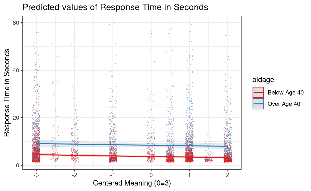
>#
># [[3]]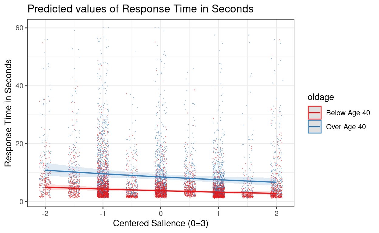
>#
># [[4]]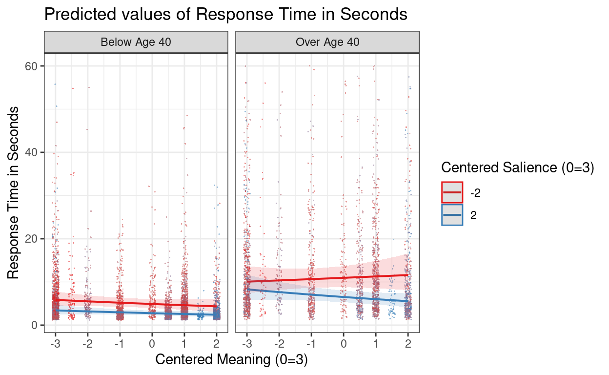
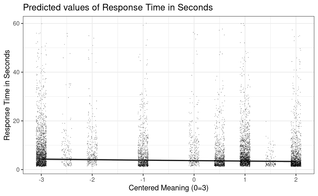
Plot the marginal age effect
# plot_model() function is from the `sjPlot` package
plot_model(m3_rs,
    type = "pred", terms = "c_mean",
    show.data = TRUE, jitter = 0.1,
    dot.alpha = 0.5, dot.size = 0.1
)
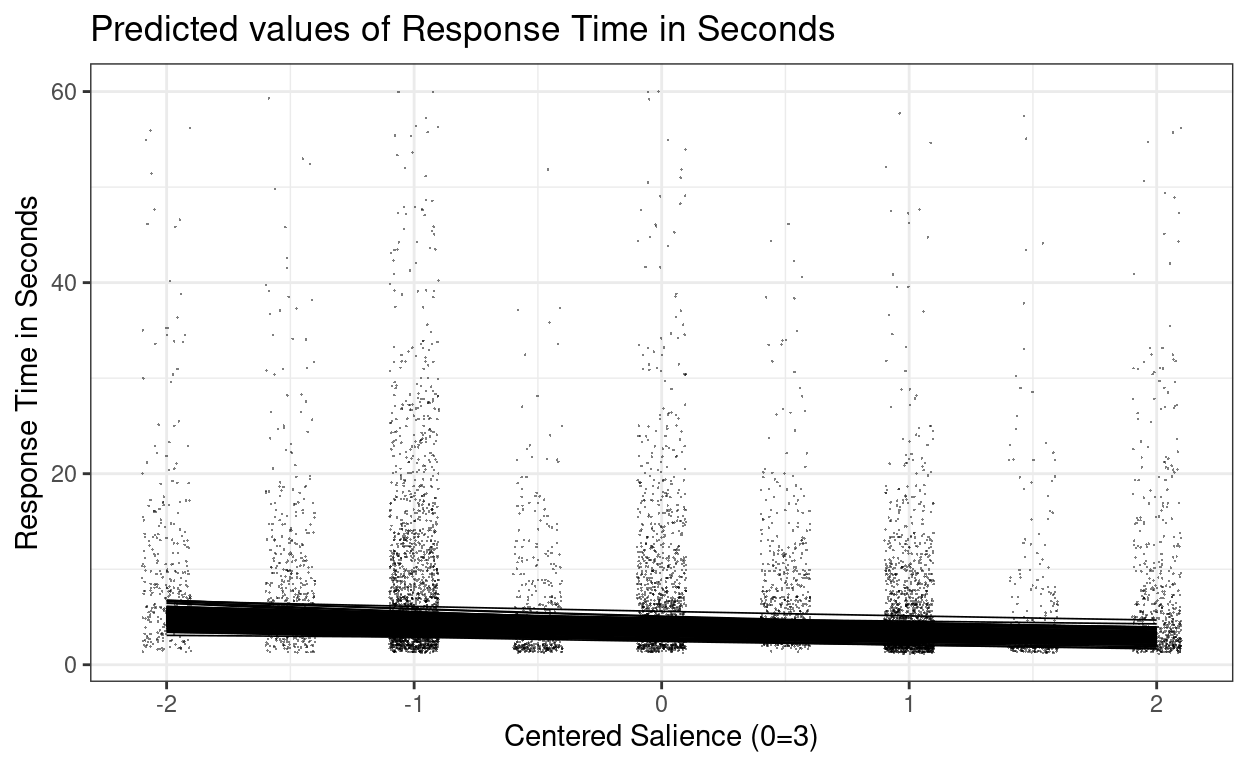
# Plot random slopes
plot_model(m3_rs,
    type = "pred",
    terms = c("c_sal", "id [1:274]"),
    pred.type = "re", show.legend = FALSE,
    colors = "black", line.size = 0.3,
    show.data = TRUE, jitter = 0.1,
    dot.alpha = 0.5, dot.size = 0.1,
    # suppress confidence band
    ci.lvl = NA
)
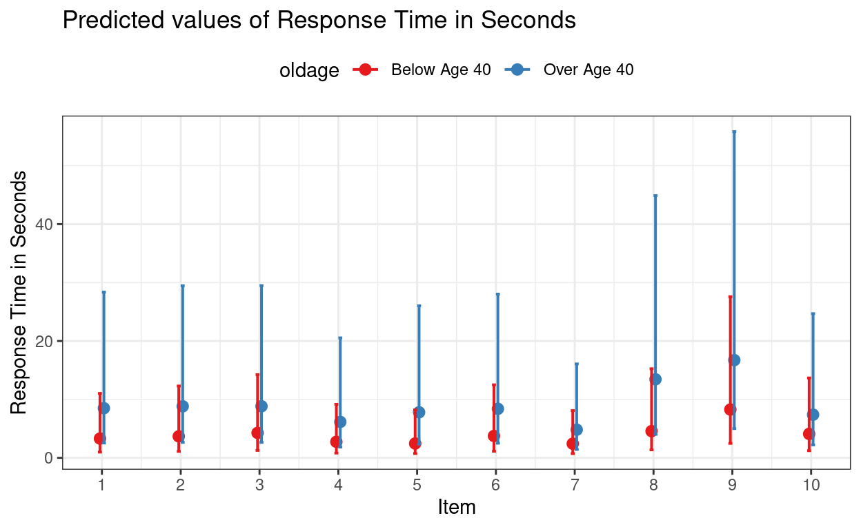
# Plot first 10 items
plot_model(m3_rs,
    type = "pred",
    terms = c("Item [1:10]", "oldage"),
    pred.type = "re"
) +
    theme(legend.position = "top")
Predicted Value for Specified Conditions
One thing that students or researchers usually want to get when reporting results is to obtain the model predictions for different experimental conditions. With our example there were three predictors, so we can get predictions for different combinations of value on the three predictors. For example, one may be interested in the following levels:
c_mean: -3 vs. 2c_sal: -2 vs. 2oldage: Below Age 40 vs. Over Age 40
You can of course obtain predictions with the equations, and that’s
the most reliable way in many cases (as long as you double and triple
check your calculations). However, with lme4, you can also
use the predict() function and specify a data frame with
all the combinations.
# Create data frame for prediction;
# the `crossing()` function generates all combinations of the input levels
pred_df <- crossing(
    c_mean = c(-3, 2),
    c_sal = c(-2, 2),
    oldage = c("Below Age 40", "Over Age 40")
)
# Add predicted values (log rt)
pred_df %>%
    mutate(
        .predicted = predict(m3_rs,
            # "newdata = ." means using the current data
            newdata = .,
            # "re.form = NA" means to not use random effects for prediction
            re.form = NA
        )
    )
># # A tibble: 8 × 4
>#   c_mean c_sal oldage       .predicted
>#    <dbl> <dbl> <chr>             <dbl>
># 1     -3    -2 Below Age 40      1.72
># 2     -3    -2 Over Age 40       2.53
># 3     -3     2 Below Age 40      1.20
># 4     -3     2 Over Age 40       2.00
># 5      2    -2 Below Age 40      1.47
># 6      2    -2 Over Age 40       2.27
># 7      2     2 Below Age 40      0.943
># 8      2     2 Over Age 40       1.75
Marginal Means
While the predict() function is handy, it requires users
to specify values for each predictor. Sometimes researchers may simply
be interested in the predicted means for levels of one or two
predictors, while averaging across other predictors in the
model. When one is averaging across one or more variables, the
predicted means are usually called the marginal means. In this case, the
emmeans package will be handy.
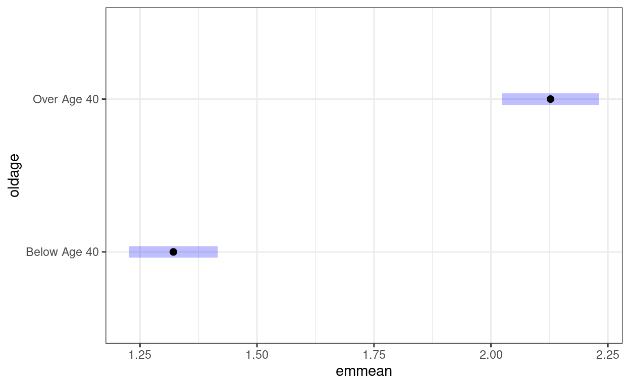
For example, suppose we are interested in only the marginal means for those below age 40 and those above age 40. We can use the following:
(emm_m3_rs <- emmeans(m3_rs, specs = "oldage", weights = "cell"))
>#  oldage       emmean     SE  df asymp.LCL asymp.UCL
>#  Below Age 40   1.32 0.0484 Inf      1.23      1.42
>#  Over Age 40    2.13 0.0530 Inf      2.02      2.23
>#
># Degrees-of-freedom method: asymptotic
># Results are given on the log (not the response) scale.
># Confidence level used: 0.95
# Plotting the means
plot(emm_m3_rs)
You can also obtain the marginal means for the transformed response variable. For example, because our response variable is log(rt), we can obtain the marginal means for the original response time variable:
emmeans(m3_rs, specs = "oldage", weights = "cell", type = "response")
>#  oldage       response    SE  df asymp.LCL asymp.UCL
>#  Below Age 40     3.75 0.181 Inf      3.41      4.12
>#  Over Age 40      8.39 0.445 Inf      7.57      9.31
>#
># Degrees-of-freedom method: asymptotic
># Confidence level used: 0.95
># Intervals are back-transformed from the log scale
Effect Size
You can compute \(R^2\). Using the additive model, the overall \(R^2\) is
MuMIn::r.squaredGLMM(m3_rs)
>#         R2m    R2c
># [1,] 0.2661 0.4603
With counterbalancing, the item-level (c_mean and
c_sal) and the person-level (oldage)
predictors are orthogonal, so we can get an \(R^2\) for the item-level predictors and an
\(R^2\) for the person-level predictor,
and they should add up approximately to the total \(R^2\). For example:
# Person-level (oldage)
m3_rs_oldage <- lmer(log(rt_sec) ~ oldage + (1 | id) +
                       (oldage | Item), data = driving_dat)
r.squaredGLMM(m3_rs_oldage)
>#         R2m    R2c
># [1,] 0.2169 0.4551
# Item-level (salience + meaning)
m3_rs_sal_mean <- lmer(log(rt_sec) ~ c_sal + c_mean + (c_sal | id) +
(1 | Item), data = driving_dat)
r.squaredGLMM(m3_rs_sal_mean)
>#          R2m    R2c
># [1,] 0.05162 0.4465
The two above adds up close to the total \(R^2\). However, c_sal and
c_mean are positively correlated, so their individual
contributions to the \(R^2\) would not
add up to the value when both are included (as there are some overlap in
their individual \(R^2\)). In this
case, you can still report the individaul \(R^2\), but remember to also report the
total.
# Salience only
m3_rs_sal <- lmer(log(rt_sec) ~ c_sal + (c_sal | id) +
                         (1 | Item), data = driving_dat)
r.squaredGLMM(m3_rs_sal)
>#          R2m    R2c
># [1,] 0.03857 0.4451
# Meaning only
m3_rs_mean <- lmer(log(rt_sec) ~ c_mean + (1 | id) +
(1 | Item), data = driving_dat)
r.squaredGLMM(m3_rs_mean)
>#          R2m    R2c
># [1,] 0.02354 0.4414
As a final word on effect size, the \(R^2\)s presented above are analogous to the \(\eta^2\) effect sizes in ANOVA.
Diagnostics
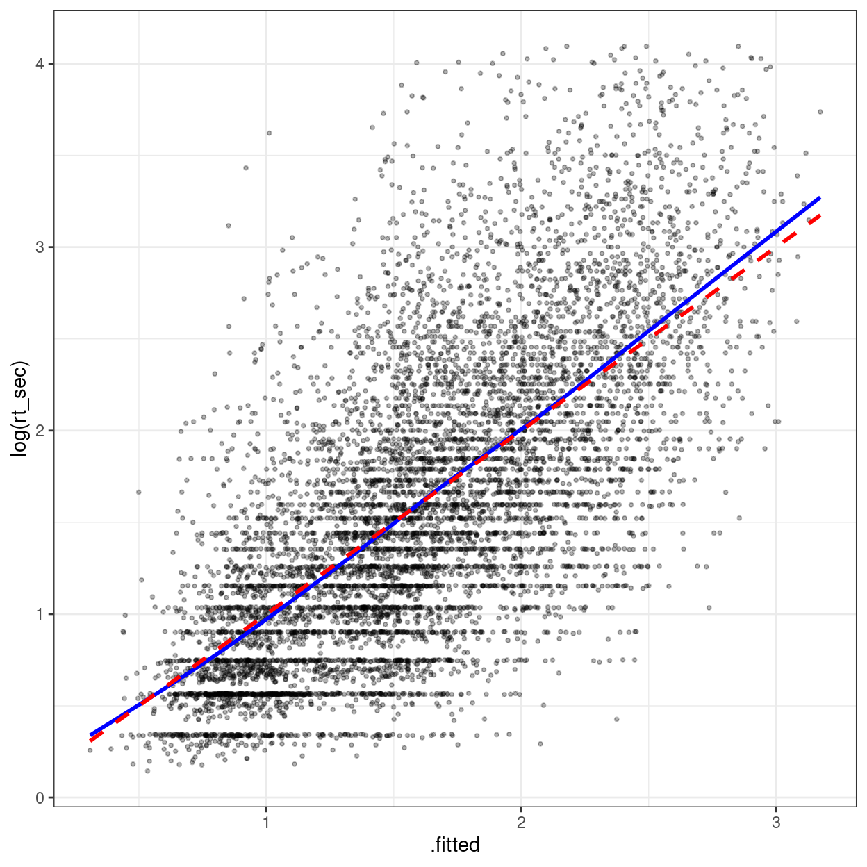
Marginal model plots
# Some discrepancy
broom.mixed::augment(m3_rs) %>%
    ggplot(aes(x = .fitted, y = `log(rt_sec)`)) +
    geom_point(size = 0.7, alpha = 0.3) +
    geom_smooth(col = "blue", se = FALSE) + # blue line from data
    geom_smooth(aes(y = .fitted),
        col = "red",
        se = FALSE, linetype = "dashed"
    ) # red line from model
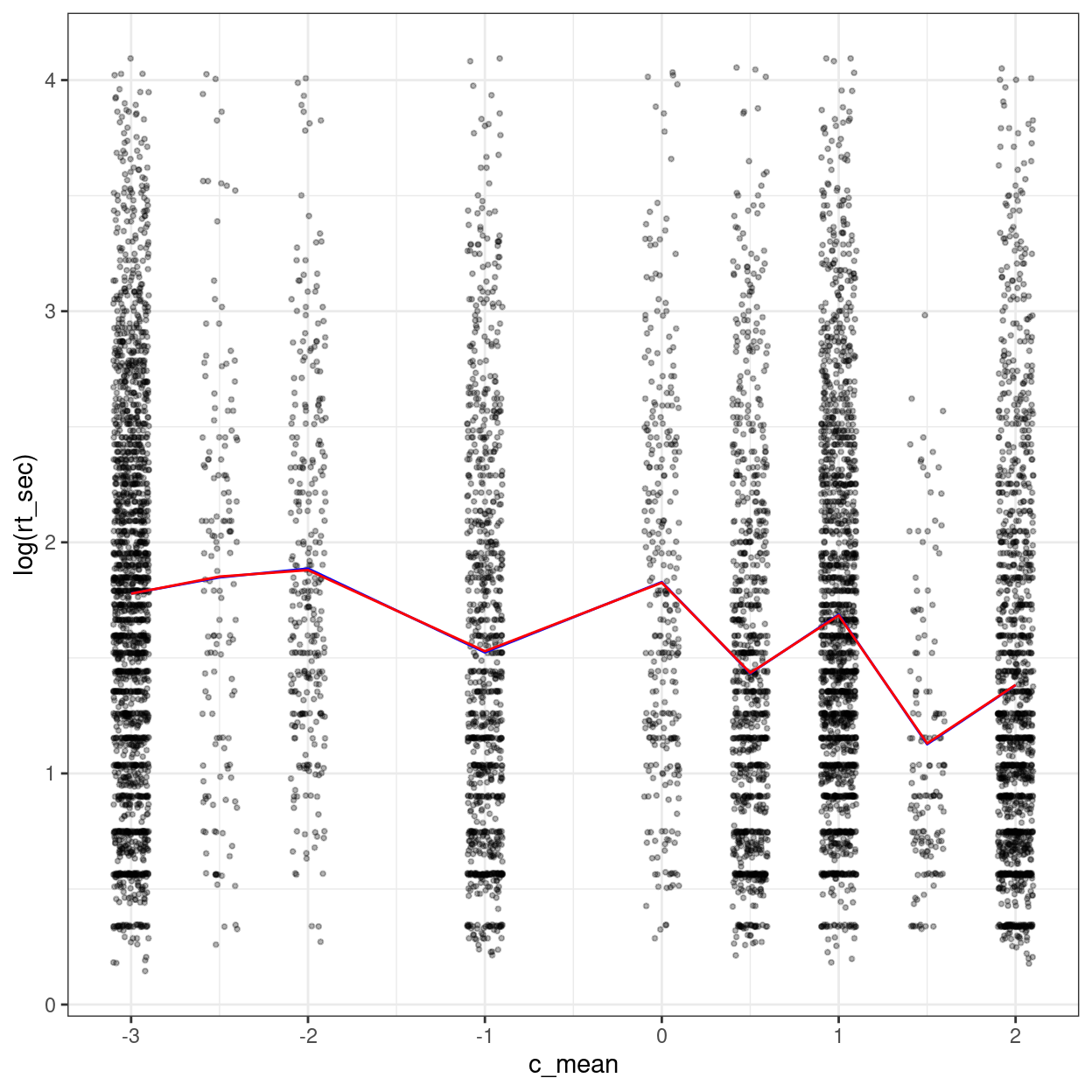
# c_mean
broom.mixed::augment(m3_rs) %>%
    ggplot(aes(x = c_mean, y = `log(rt_sec)`)) +
    geom_jitter(size = 0.7, alpha = 0.3, width = 0.1) +
    stat_summary(
        fun = mean, col = "blue",
        geom = "line"
    ) + # blue line from data
    stat_summary(aes(y = .fitted),
        fun = mean, col = "red",
        geom = "line"
    ) # red line from model
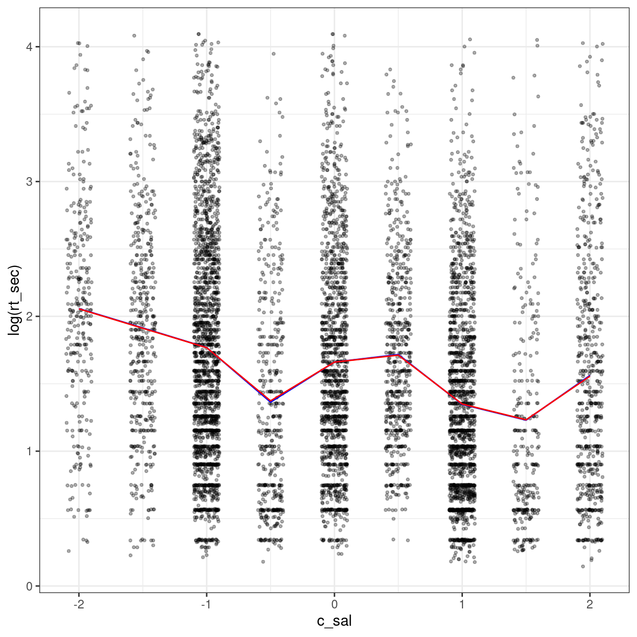
# c_sal
broom.mixed::augment(m3_rs) %>%
    ggplot(aes(x = c_sal, y = `log(rt_sec)`)) +
    geom_jitter(size = 0.7, alpha = 0.3, width = 0.1) +
    stat_summary(
        fun = mean, col = "blue",
        geom = "line"
    ) + # blue line from data
    stat_summary(aes(y = .fitted),
        fun = mean, col = "red",
        geom = "line"
    ) # red line from model
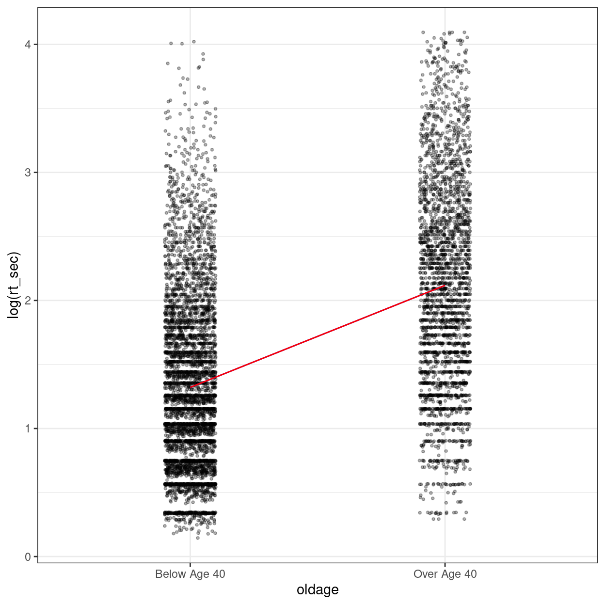
# oldage
broom.mixed::augment(m3_rs) %>%
    ggplot(aes(x = oldage, y = `log(rt_sec)`)) +
    geom_jitter(size = 0.7, alpha = 0.3, width = 0.1) +
    stat_summary(
        aes(group = 1),
        fun = mean, col = "blue",
        geom = "line"
    ) + # blue line from data
    stat_summary(aes(y = .fitted, group = 1),
        fun = mean, col = "red",
        geom = "line"
    ) # red line from model
Residual Plots
broom.mixed::augment(m3_rs) %>%
    mutate(.std_resid = resid(m3_rs, scaled = TRUE)) %>%
    ggplot(aes(x = .fitted, y = .std_resid)) +
    geom_point(size = 0.7, alpha = 0.5) +
    geom_smooth(se = FALSE)
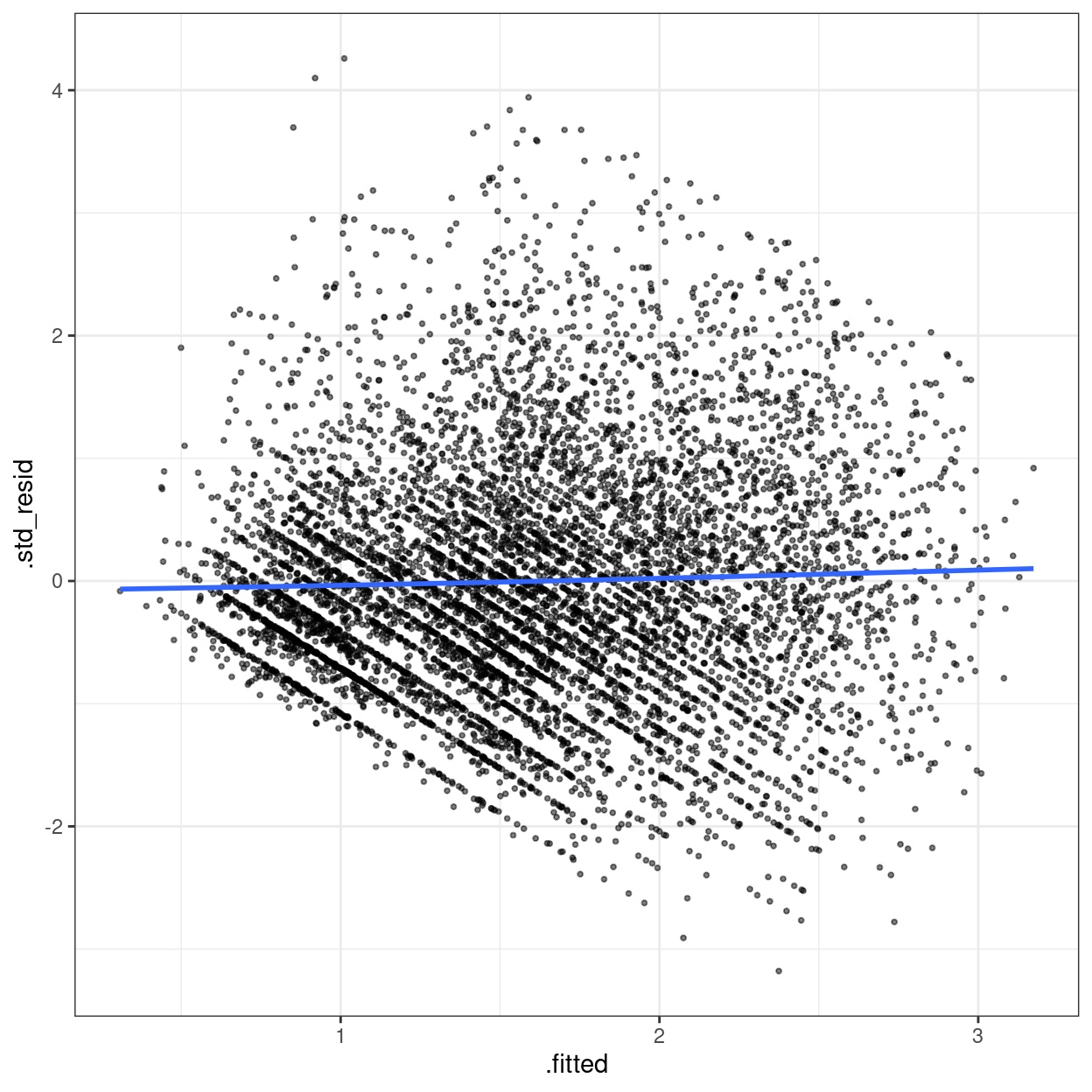
You can see some boundary in bottom left of the graph, which is due to the outcome being non-negative.