\[ \newcommand{\bv}[1]{\boldsymbol{\mathbf{#1}}} \]
Click here to download the Rmd file: week6-mlm-diagnostic.Rmd
In R, there are many quite a few diagnostic tools for MLM, although they are not necessarily straightforward to use. In this note I will show some basic tools.
Load Packages and Import Data
# To install a package, run the following ONCE (and only once on your computer)
# install.packages("psych")
library(here)  # makes reading data more consistent
library(tidyverse)  # for data manipulation and plotting
library(haven)  # for importing SPSS/SAS/Stata data
library(lme4)  # for multilevel analysis
library(lmerTest)  # for testing in small samples
library(splines)  # for nonlinear trend
library(broom.mixed)  # for getting predicted values/residuals
library(modelsummary)  # for plotting
theme_set(theme_bw())  # Theme; just my personal preference
Here’s a function I created for marginal model plots
mmps_lmer <- function(object) {
  plot_df <- object@frame
  form <- formula(object)
  xvar <- attr(attr(plot_df, "terms"), "varnames.fixed")[-1]
  plot_df$.fitted_x <- fitted(object)
  plot_df$.fitted <- plot_df$.fitted_x
  plot_df$.rowid <- seq_len(nrow(plot_df))
  plot_df_long <- reshape(plot_df, direction = "long",
                          varying = c(xvar, ".fitted_x"),
                          v.names = "xvar",
                          idvar = ".rowid")
  plot_df_long$varname <- rep(c(xvar, ".fitted"),
                              each = nrow(plot_df))
  ggplot(
    data = plot_df_long,
    aes_string(x = "xvar", y = paste(form[[2]]))
  ) +
    geom_point(size = 0.5, alpha = 0.3) +
    geom_smooth(aes(col = "data"), se = FALSE) +
    geom_smooth(aes(y = .fitted, col = "model"),
      linetype = "dashed", se = FALSE
    ) +
    facet_wrap(~ varname, scales = "free_x") +
    labs(color = NULL, x = NULL) +
    scale_color_manual(values = c("data" = "blue",
                                  "model" = "red")) +
    theme(legend.position = "bottom")
}
# Read in the data (pay attention to the directory)
hsball <- read_sav(here("data_files", "hsball.sav"))
# Cluster-mean centering
hsball <- hsball %>%
  group_by(id) %>%  # operate within schools
  mutate(ses_cm = mean(ses),  # create cluster means (the same as `meanses`)
         ses_cmc = ses - ses_cm) %>%  # cluster-mean centered
  ungroup()  # exit the "editing within groups" mode
The discussion will follow chapter 10 of Snijders & Bosker (2012)
Fitting the model
We will first use a model with ses and
sector, without contextual effects or random slopes.
m1 <- lmer(mathach ~ sector + ses + (1 | id),
           data = hsball)
Diagnostics
Does the fixed part contain the right variables?
Cluster means for lower-level variables
One can test whether ses_cm should be included in the
model, in addition to the raw level-1 variable. Let’s use likelihood
ratio tests for it:
>#               2.5 % 97.5 %
># .sig01       1.3013  1.769
># .sigma       5.9850  6.186
># (Intercept) 11.7392 12.517
># sector       0.6268  1.822
># ses          1.9782  2.404
># ses_cm       2.3942  3.896
So it looks like we need ses_cm.
Omitted variables
If there are any potential confounding variable, those should be included as well. This requires knowledge of the research question under investigation. One good thing is that if one is interested in effects at a lower level, doing cluster-mean centering or including the cluster mean will rule out potential confounders at a higher level. This is because one is now comparing individuals within the same school (or the same level-2 unit), so any confounders that are related to school characteristics can be ruled out, as they will be held constant.
Linearity
A quick way to check whether there are any unmodelled non-linear trends is to use marginal model plots, which shows the outcome variable against each individual predictor. The plot shows two lines: one shows a nonparametric smoother that does not depend on the model, and the other shows the implied association based on the model. If the two lines are close to each other, then there is no need to include extra curvillinear terms of the predictors; otherwise, one may need to consider adding quadratic or other non-linear terms.
m2 <- lmer(mathach ~ sector + ses + ses_cm + (1 | id),
  data = hsball
)
# SES
augment(m2) %>%
  ggplot(aes(x = ses, y = mathach)) +
  geom_point(size = 0.7, alpha = 0.3) +
  geom_smooth(col = "blue", se = FALSE) + # blue line from data
  geom_smooth(aes(y = .fitted),
    col = "red",
    se = FALSE, linetype = "dashed"
  )  # red line from model
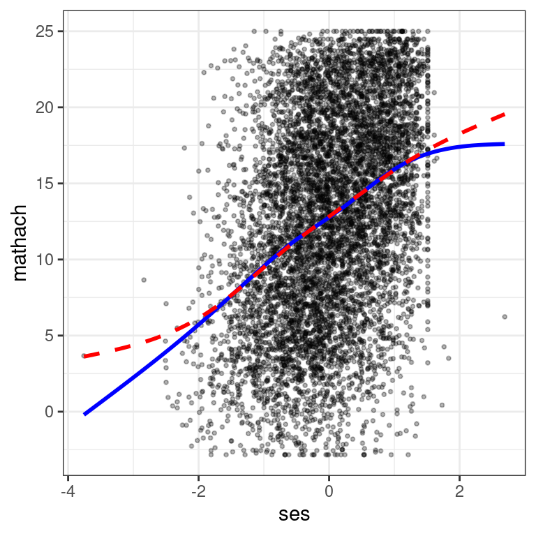
The above shows some deviation between the model (red line) and the
data (blue line), but the discrepancy is mostly driven by two data
points, one on the left and one on the right. So this is mostly fine,
although it is possible to check whether the results are similar without
those two points. You can modify the code to check all other predictors
as well. To make things easier, I’ve made a small function,
mmps_lmer(), defined in the beginning of the file, that
automatically generates the marginal model plots for all predictors:
mmps_lmer(m2)
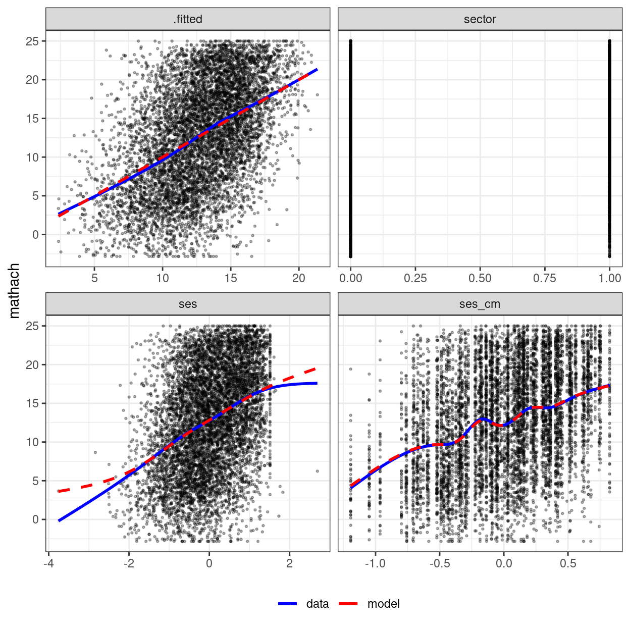
There are two things to note. First, for binary predictors
female and sector, the plot is not meaningful,
as there are only two possible values in the predictor. Second, the plot
labelled .fitted is one where it plots the outcome against
the linear precictor, which is the predicted value of the
outcome based on the predictors (i.e., \(\gamma_{00} + \gamma_{01}\)). You can think
about it as a combination of all predictors.
To show what it is like when linearity is violated, I simulate some data by adding a quadratic term:
## Fake example: Add quadratic trend for ses
hsball_quad <- hsball %>%
  mutate(mathach = mathach + ses^2)
m2_quad <- refit(m2, newresp = hsball_quad$mathach)
mmps_lmer(m2_quad)
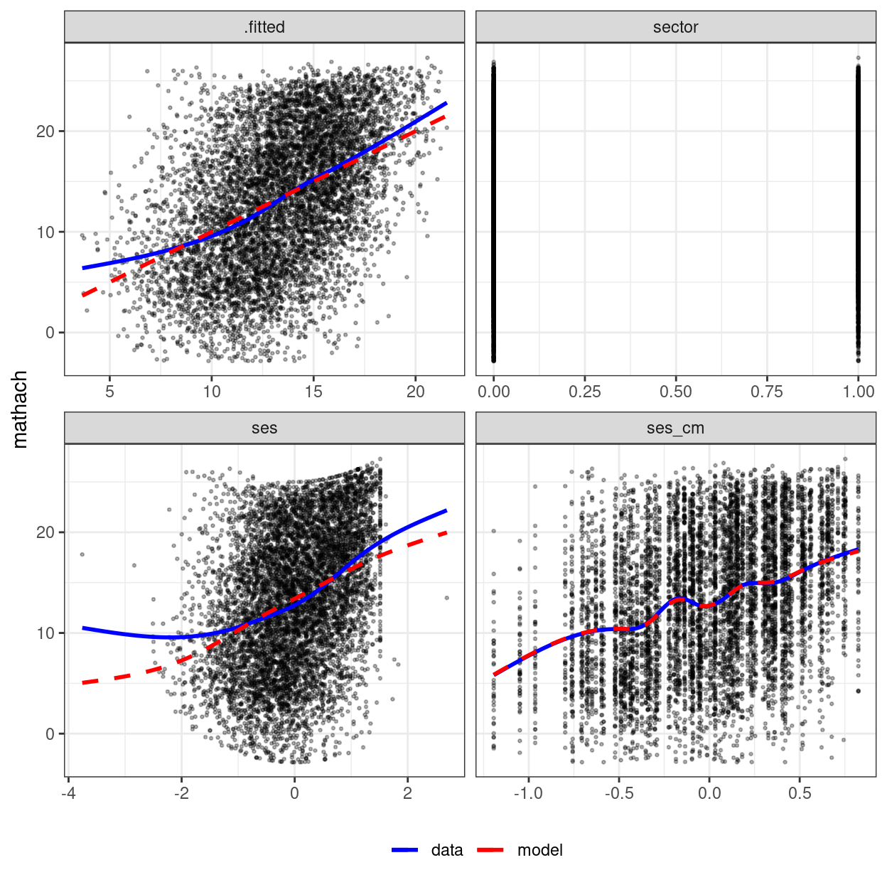
The above shows a misfit for the plot with ses.
What to do if linearity is violated?
- Include non-linear terms (e.g., quadratic)
- Include interactions (but note that interactions can be present even when linearity is not violated)
- Using splines. Below is an example:
# Need the `spline` package; bs() for cubic spline
m2_spline <- lmer(mathach ~ sector + bs(ses) + bs(ses_cm) + (1 | id),
  data = hsball
)
# See whether nonlinear trend is needed
anova(m2, m2_spline)  # not statistically significant
># Data: hsball
># Models:
># m2: mathach ~ sector + ses + ses_cm + (1 | id)
># m2_spline: mathach ~ sector + bs(ses) + bs(ses_cm) + (1 | id)
>#           npar   AIC   BIC logLik deviance Chisq Df Pr(>Chisq)
># m2           6 46560 46602 -23274    46548
># m2_spline   10 46565 46634 -23273    46545  3.31  4       0.51
# So insufficient evidence for a nonlinear trend for `ses` and `ses_cm`
Does the random part contain the right variables?
Testing for random slopes
># ANOVA-like table for random-effects: Single term deletions
>#
># Model:
># mathach ~ sector + ses + ses_cm + (ses | id)
>#                   npar logLik   AIC  LRT Df Pr(>Chisq)
># <none>               8 -23274 46563
># ses in (ses | id)    6 -23277 46566 6.36  2      0.042 *
># ---
># Signif. codes:  0 '***' 0.001 '**' 0.01 '*' 0.05 '.' 0.1 ' ' 1
The random slope for ses was significant, so it should
be included.
Residual Plots
Residuals can be used to check a lot of assumptions, including linearity, homoscedasticity, normality, and outliers
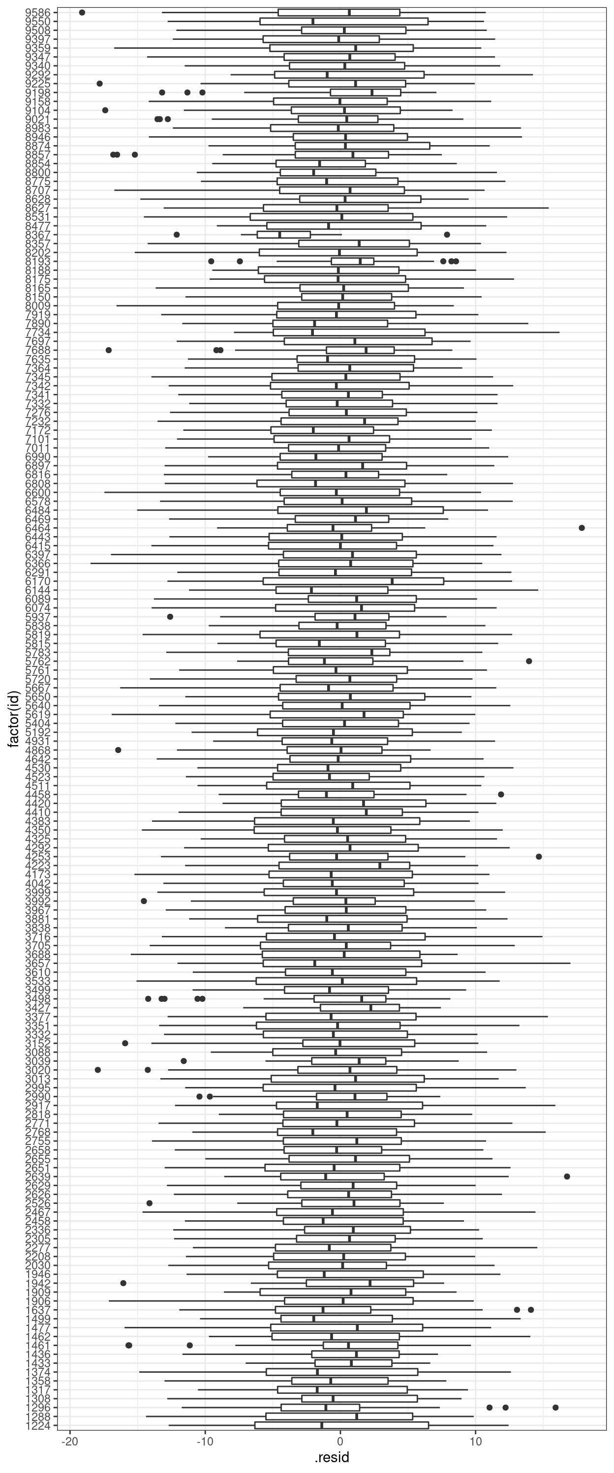
Residuals across clusters
The following computes the standardized residuals and plot them across different clusters. The following plot shows:
- Most of the standardized residuals are between -3 and 3, so not a lot of outliers;
- The variability of the residuals is similar across clusters, so heteroscedastisticity is likely not an issue across clusters.
augment(m3) %>%
  ggplot(aes(x = factor(id), y = .resid)) +
  geom_boxplot() +
  coord_flip()
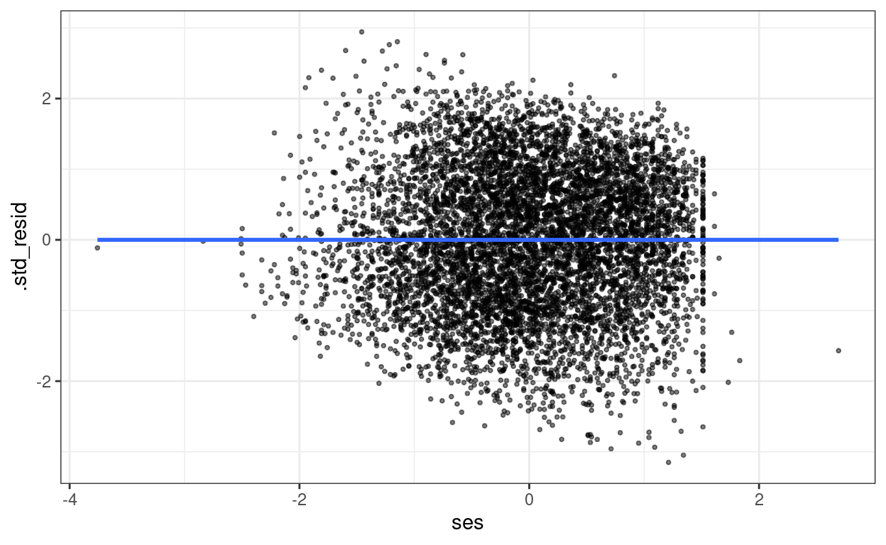
Level-1 residuals across predictors
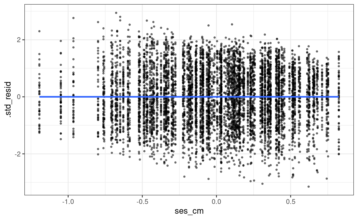
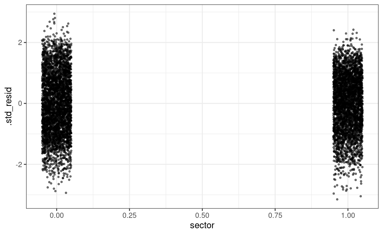
The plot below shows that heteroscedastisticity is likely not a problem, as we do not see clearly bigger/smaller variance at certain levels of the predictors.
augment(m3) %>%
  mutate(.std_resid = resid(m3, scaled = TRUE)) %>%
  ggplot(aes(x = ses, y = .std_resid)) +
  geom_point(size = 0.7, alpha = 0.5) +
  geom_smooth(se = FALSE)
augment(m3) %>%
  mutate(.std_resid = resid(m3, scaled = TRUE)) %>%
  ggplot(aes(x = ses_cm, y = .std_resid)) +
  geom_point(size = 0.7, alpha = 0.5) +
  geom_smooth(se = FALSE)
augment(m3) %>%
  mutate(.std_resid = resid(m3, scaled = TRUE)) %>%
  ggplot(aes(x = sector, y = .std_resid)) +
  # use `geom_jitter` for discrete predictor
  geom_jitter(size = 0.7, alpha = 0.5, width = 0.05)
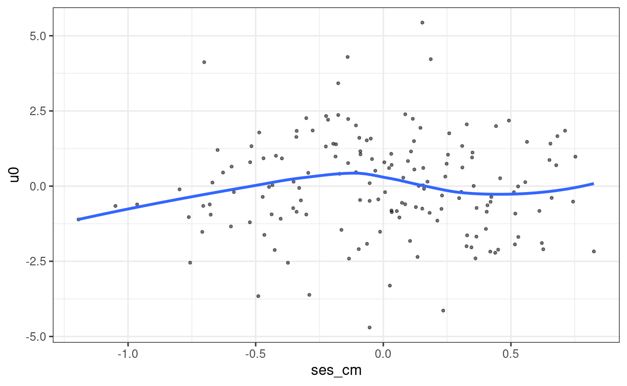
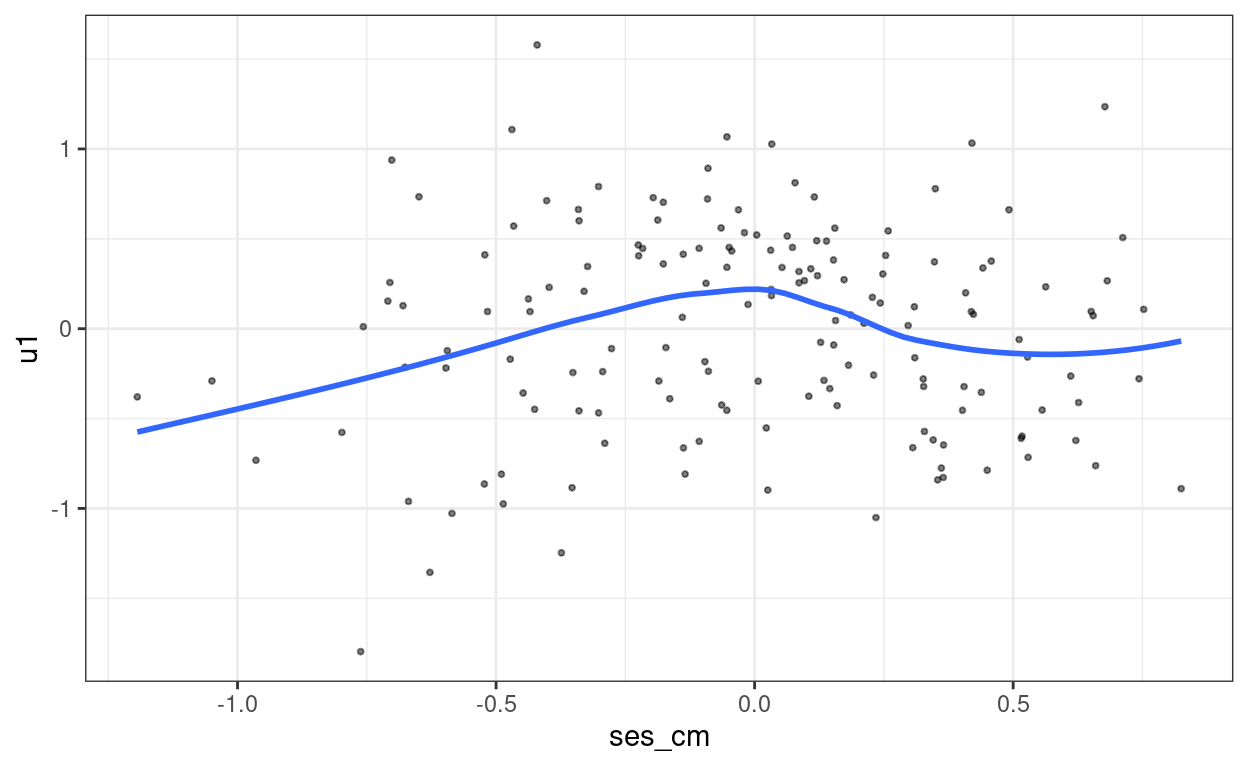
Level-2 residuals across lv-2 predictors
resid_lv2 <- ranef(m3)$id
resid_lv2_var <- attr(resid_lv2, "postVar")
resid_lv2_sd <- sqrt(cbind(
  resid_lv2_var[1, 1, ],
  resid_lv2_var[2, 2, ]
))
std_resid_lv2 <- resid_lv2 %>%
  rownames_to_column("id") %>%
  transmute(id = id,
            u0 = `(Intercept)` / resid_lv2_sd[, 1],
            u1 = ses / resid_lv2_sd[, 2])
# Merge lv-2 data with lv-2 standardized residuals
hsball_lv2 <- hsball %>%
  group_by(id) %>%
  summarise(ses_cm = ses_cm[1]) %>%
  left_join(
    std_resid_lv2
  )
# Plot lv-2 residual against `ses_cm`
ggplot(hsball_lv2, aes(x = ses_cm, y = u0)) +
  geom_point(size = 0.7, alpha = 0.5) +
  geom_smooth(se = FALSE)
ggplot(hsball_lv2, aes(x = ses_cm, y = u1)) +
  geom_point(size = 0.7, alpha = 0.5) +
  geom_smooth(se = FALSE)
Bonus: Modeling heteroscedastisticity
You can model \(\log(\sigma_{ij}) = \gamma^{s}_{00} + \gamma^{s}_{10} x_{ij} + \gamma^{s}_{01} w_{j}\)
Let’s model the variance as a function of sector.
library(glmmTMB)
# Assume homoscedasticity
m3_tmb <- glmmTMB(mathach ~ sector + ses + ses_cm + (ses | id),
  data = hsball
)
# Modeling heteroscedasticity
m3_heter_tmb <- glmmTMB(
  mathach ~ sector + ses + ses_cm + (ses | id),
  dispformula = ~ sector,  # difference variance for different sectors
  data = hsball
)
summary(m3_heter_tmb)  # catholic school has a larger variance
>#  Family: gaussian  ( identity )
># Formula:          mathach ~ sector + ses + ses_cm + (ses | id)
># Dispersion:               ~sector
># Data: hsball
>#
>#      AIC      BIC   logLik deviance df.resid
>#    46531    46593   -23257    46513     7176
>#
># Random effects:
>#
># Conditional model:
>#  Groups   Name        Variance Std.Dev. Corr
>#  id       (Intercept) 2.372    1.540
>#           ses         0.458    0.677    0.21
>#  Residual                NA       NA
># Number of obs: 7185, groups:  id, 160
>#
># Conditional model:
>#             Estimate Std. Error z value Pr(>|z|)
># (Intercept)   12.068      0.219    55.1  < 2e-16 ***
># sector         1.353      0.361     3.7  0.00018 ***
># ses            2.148      0.123    17.5  < 2e-16 ***
># ses_cm         3.217      0.398     8.1  6.5e-16 ***
># ---
># Signif. codes:  0 '***' 0.001 '**' 0.01 '*' 0.05 '.' 0.1 ' ' 1
>#
># Dispersion model:
>#             Estimate Std. Error z value Pr(>|z|)
># (Intercept)   3.6913     0.0239   154.4   <2e-16 ***
># sector       -0.1833     0.0340    -5.4    7e-08 ***
># ---
># Signif. codes:  0 '***' 0.001 '**' 0.01 '*' 0.05 '.' 0.1 ' ' 1
# Compare the two models
anova(m3_tmb, m3_heter_tmb) # the heteroscedastic model has a better deviance
># Data: hsball
># Models:
># m3_tmb: mathach ~ sector + ses + ses_cm + (ses | id), zi=~0, disp=~1
># m3_heter_tmb: mathach ~ sector + ses + ses_cm + (ses | id), zi=~0, disp=~sector
>#              Df   AIC   BIC logLik deviance Chisq Chi Df Pr(>Chisq)
># m3_tmb        8 46558 46613 -23271    46542
># m3_heter_tmb  9 46531 46593 -23257    46513    29      1    7.2e-08
>#
># m3_tmb
># m3_heter_tmb ***
># ---
># Signif. codes:  0 '***' 0.001 '**' 0.01 '*' 0.05 '.' 0.1 ' ' 1
# The fixed effects are pretty comparable
msummary(list(
`Homoscedastic` = m3_tmb,
`Heteroscedastic` = m3_heter_tmb
))
| Homoscedastic | Heteroscedastic | |
|---|---|---|
| (Intercept) | 12.044 | 12.068 |
| (0.216) | (0.219) | |
| sector | 1.409 | 1.353 |
| (0.360) | (0.361) | |
| ses | 2.196 | 2.148 |
| (0.122) | (0.123) | |
| ses_cm | 3.151 | 3.217 |
| (0.396) | (0.398) | |
| sd__(Intercept) | 1.538 | 1.540 |
| sd__ses | 0.675 | 0.677 |
| cor__(Intercept).ses | 0.276 | 0.205 |
| sd__Observation | 6.065 | |
| Num.Obs. | 7185 | 7185 |
| AIC | 46558.3 | 46531.3 |
| BIC | 46613.3 | 46593.2 |
| Log.Lik. | −23271.137 | −23256.632 |
Bonus: Heteroscedasticity-consistent (HC) variance estimates
If you suspect that heteroscedastisticity may be a problem, you can
also use the heteroskedasticity-consistent variance estimators with the
clubSandwich package, which computes the HC correction for
the test results
library(clubSandwich)
# Sampling variances of fixed effects from REML
vcov_m3 <- vcov(m3)
# Sampling variances from HC
vcovcr_m3 <- vcovCR(m3, type = "CR2")
# Compare standard errors: REML-SE and HC-SE
cbind(
  "REML-SE" = sqrt(diag(vcov_m3)),
  "HC-SE" = sqrt(diag(vcovcr_m3))
)
>#             REML-SE  HC-SE
># (Intercept)  0.2017 0.1780
># sector       0.3091 0.3158
># ses          0.1224 0.1288
># ses_cm       0.3881 0.3660
# Testing fixed effects adjusting for heteroscedasticity
coef_test(m3, vcov = "CR2")
>#        Coef. Estimate    SE t-stat d.f. (Satt) p-val (Satt) Sig.
>#  (Intercept)    12.04 0.178  67.66        84.8       <0.001  ***
>#       sector     1.41 0.316   4.46        99.0       <0.001  ***
>#          ses     2.20 0.129  17.05       146.9       <0.001  ***
>#       ses_cm     3.16 0.366   8.62        62.2       <0.001  ***
Note: To my knowledge, currently it is not possible to combine HC estimator with the small-sample Kenward-Roger correction.
Q-Q Plot for Lv-1 Residuals
For: normality
You want to see the points line up nicely along the 45 degree line
library(lattice)  # need this package to use the built-in functions
qqmath(m3)  # just use the `qqmath()` function on the fitted model
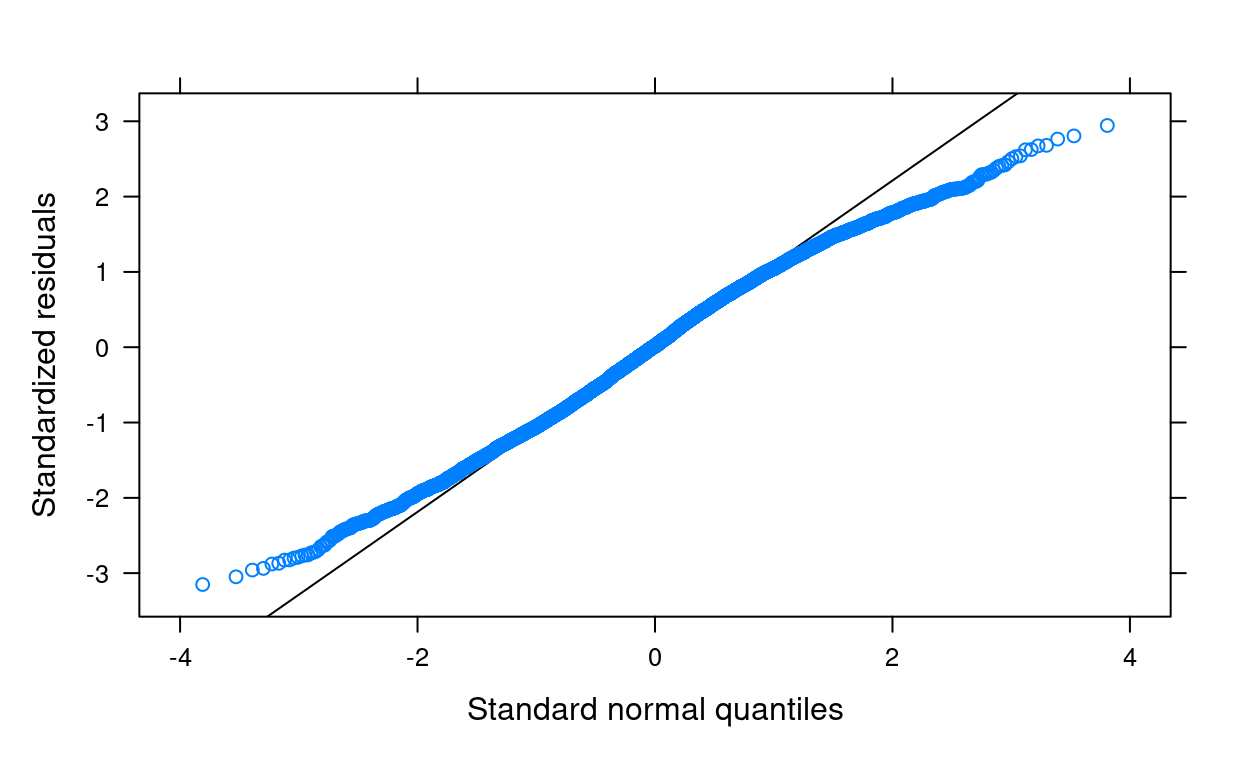
There are some deviations from normality on the two tail areas, which is likely due to less kurtosis because of the boundedness of the outcome variable. Generally the impact of kurtosis is not as severe as skewness, and the above plot did not suggest a major issue to the results.
Q-Q Plot for Lv-2 Residuals
For: normality
At level 2 there can be more then one set of residuals. For example, in this model, we have one set for the random intercept, and the other set for the random slope
# the code is a bit more complex in order to add the reference line, but you
# only need to replace `m3` with the name of your own model to get the
# plots for your own analyses
qqmath(ranef(m3, condVar = FALSE),
       panel = function(x) {
         panel.qqmath(x)
         panel.qqmathline(x)
       })
># $id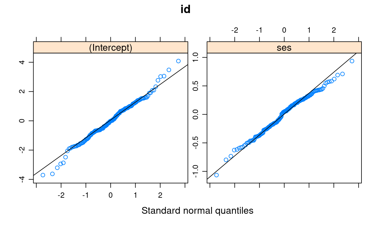
Normality does not appear to be an issue at level 2.
Bonus: Variance Inflation Factor (VIF)
For: multicollinearity
As a rule of thumb, one would worry about multicollinearity in the predictors when VIF > 4, and VIF > 10 indicates strong multicollinearity.
Bonus: Influence Index Plots
For: leverage points and outliers
To examine whether some cases gives disproportionately strong influence on the results, we can look at influence index plot and dfbeta
# It seems that the influence() function only supports object of class `data.frame`, so we need to
# change the data class and refit the model
hsball_2 <- as.data.frame(hsball)
m3_2 <- lmer(mathach ~ sector + ses + ses_cm + (ses | id),
           data = hsball_2)
inf_m3 <- influence(m3_2, "id")  # get cluster-level influence statistics
car::infIndexPlot(inf_m3)
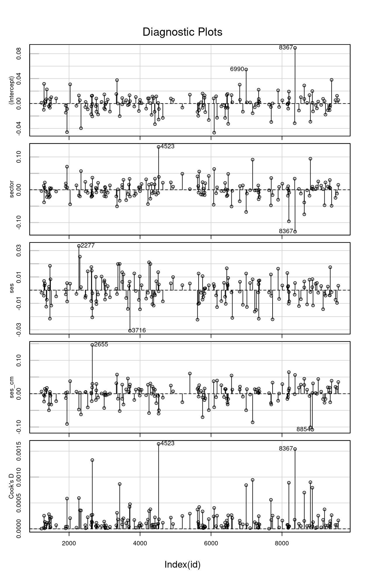
If you need some cutoffs, the cutoff for dfbeta is \(2 / \sqrt{job}\), which would be 0.1581 in our example; cutoff for Cook’s distance is \(4 / (J - 2)\), which would be 0.0253 in our example. So while some of the clusters exert more influence on the results than others, they all seem to be within the normal sampling variability that one would expect. If some clusters are above the cutoffs, then you may want to take a look on those clusters to see whether there are coding errors, or whether there is something unique about them. You can do a sensitivity analysis with and without those clusters.
Bonus: Bayesian Robust MLM
There has not been a lot of discussion on MLM that is robust to
outliers. One useful technique, however, is to use a heavy-tailed
distribution for the errors and random effects. Instead of assuming that
they follow normal distributions, we assume them to follow Student’s
\(t\) distributions, which have heavier
tails. What it does is to allow for a higher probability of extreme
value, so that those extreme values will have less influence on
estimating the pattern of the data. You will need to use the
brms package. The installation of this package, however, is
not straightforward (https://github.com/paul-buerkner/brms), so if you are
not able to run it here, don’t worry as we don’t need it for the
remainder of the class.
library(brms)
# Same syntax; just change `lmer()` to `brm()`
m3_robust <- brm(
  mathach ~ sector + ses + ses_cm +
    # Assume random effects follow a t distribution
    (ses | gr(id, dist = "student")),
  # Assume the errors follow a t distribution
  family = student(),
  data = hsball,
  chains = 2,
  control = list(adapt_delta = .95)
)
The results are similar, so the regular MLM should be fine here
| Normal MLM | Robust MLM | |
|---|---|---|
| (Intercept) | 12.043 | 12.083 |
| (0.202) | (0.217) | |
| sector | 1.408 | 1.342 |
| (0.309) | (0.359) | |
| ses | 2.196 | 2.215 |
| (0.122) | (0.116) | |
| ses_cm | 3.155 | 3.194 |
| (0.388) | (0.403) | |
| sd__(Intercept) | 1.559 | 1.416 |
| (0.155) | ||
| cor__(Intercept).ses | 0.270 | 0.252 |
| (0.273) | ||
| sd__ses | 0.688 | 0.550 |
| (0.209) | ||
| sd__Observation | 6.065 | 6.026 |
| (0.055) | ||
| Num.Obs. | 7185 | 7185 |
| AIC | 46563.5 | |
| BIC | 46618.5 | |
| Log.Lik. | −23273.735 | |
| REMLcrit | 46547.471 | |
| algorithm | sampling | |
| pss | 2000.000 |
Convergence
It’s not uncommon to run into convergence issues when the model contains two or more random slopes, or when the sample size (i.e., number of clusters) is small.
Multiple Random Slopes
Here I include female and its random slopes
m_complex <- lmer(
  mathach ~ sector + ses + ses_cm + female + (ses + female | id),
  data = hsball
)
You will see the above warning. This almost always happens with two or more random slopes.
You can consult https://bbolker.github.io/mixedmodels-misc/glmmFAQ.html#troubleshooting regarding some suggestions on what to do (and I recommend that you save this page for your future reference).
The first thing you can do is to do centering and scaling. For scaling, it means making the predictors to have a smaller range. For example, if one of your predictor is income in dollars, I would suggest dividing income by $10,000 so that the resulting values are smaller. For centering, we can try using the cluster-mean centered variables:
m_complex2 <- lmer(
  mathach ~ sector + ses_cmc + ses_cm + female_cmc + female_cm +
    (ses_cmc + female_cmc | id),
  data = hsball
)
The warning actually goes away now. If it does not, the next thing you can do is to try a different optimizer:
m_complex_all <- lme4::allFit(m_complex)
># bobyqa : [OK]
># Nelder_Mead : [OK]
># nlminbwrap : [OK]
># nmkbw : [OK]
># optimx.L-BFGS-B : [OK]
># nloptwrap.NLOPT_LN_NELDERMEAD : [OK]
># nloptwrap.NLOPT_LN_BOBYQA : [OK]
ss <- summary(m_complex_all) # this shows everything
# Check which optimizer work
ss$which.OK
>#                        bobyqa                   Nelder_Mead
>#                          TRUE                          TRUE
>#                    nlminbwrap                         nmkbw
>#                          TRUE                          TRUE
>#               optimx.L-BFGS-B nloptwrap.NLOPT_LN_NELDERMEAD
>#                          TRUE                          TRUE
>#     nloptwrap.NLOPT_LN_BOBYQA
>#                          TRUE
# Compare the converged log-likelihood from different optimizers
ss$llik
>#                        bobyqa                   Nelder_Mead
>#                        -23314                        -23244
>#                    nlminbwrap                         nmkbw
>#                        -23244                        -23244
>#               optimx.L-BFGS-B nloptwrap.NLOPT_LN_NELDERMEAD
>#                        -23314                        -23244
>#     nloptwrap.NLOPT_LN_BOBYQA
>#                        -23244
# Compare the fixed effects
ss$fixef
>#                               (Intercept) sector   ses ses_cm female
># bobyqa                              12.81  1.279 2.160  3.105 -1.345
># Nelder_Mead                         12.67  1.377 2.155  3.075 -1.192
># nlminbwrap                          12.67  1.377 2.155  3.075 -1.192
># nmkbw                               12.67  1.377 2.155  3.075 -1.192
># optimx.L-BFGS-B                     12.81  1.279 2.160  3.105 -1.345
># nloptwrap.NLOPT_LN_NELDERMEAD       12.67  1.377 2.155  3.075 -1.192
># nloptwrap.NLOPT_LN_BOBYQA           12.67  1.377 2.155  3.075 -1.192
So it looks like the bobyqa optimizer (the default)
converge to a different solution than other optimizers. The
log-likelihood value is better (i.e., less negative) for the other
optimizers than the default, so we should try those. Let’s use
nlminbwrap
m_complex <- lmer(
  mathach ~ sector + ses + ses_cm + female + (ses + female | id),
  data = hsball,
  control = lmerControl(optimizer = "nlminbwrap")
)
The warning goes away.
Singular Models
Especially in small samples, you will run into a message of singular model fit, like
# Randomly select 10 school ids
set.seed(1059)  # use the same seed so that the same 10 schools are selected
random_ids <- sample(unique(hsball$id), size = 10)
hsbsub <- hsball %>%
    filter(id %in% random_ids)
# Fit a model
m3_small <- lmer(mathach ~ sector + ses + ses_cm + (ses | id),
                 data = hsbsub)
summary(m3_small)
># Linear mixed model fit by REML. t-tests use Satterthwaite's method [
># lmerModLmerTest]
># Formula: mathach ~ sector + ses + ses_cm + (ses | id)
>#    Data: hsbsub
>#
># REML criterion at convergence: 2799
>#
># Scaled residuals:
>#    Min     1Q Median     3Q    Max
># -2.564 -0.699 -0.035  0.748  2.887
>#
># Random effects:
>#  Groups   Name        Variance Std.Dev. Corr
>#  id       (Intercept)  3.020   1.738
>#           ses          0.244   0.494    -1.00
>#  Residual             40.135   6.335
># Number of obs: 428, groups:  id, 10
>#
># Fixed effects:
>#             Estimate Std. Error     df t value Pr(>|t|)
># (Intercept)   11.944      0.875  6.904   13.65    3e-06 ***
># sector        -1.018      1.478  6.342   -0.69  0.51551
># ses            2.247      0.473 18.902    4.75  0.00014 ***
># ses_cm         3.701      2.322  8.475    1.59  0.14753
># ---
># Signif. codes:  0 '***' 0.001 '**' 0.01 '*' 0.05 '.' 0.1 ' ' 1
>#
># Correlation of Fixed Effects:
>#        (Intr) sector ses
># sector -0.663
># ses    -0.251  0.045
># ses_cm  0.480 -0.478 -0.240
># optimizer (nloptwrap) convergence code: 0 (OK)
># boundary (singular) fit: see help('isSingular')
If you look at the random effect matrix, the correlation between the
random intercepts and the random slopes is -1, which is small. Usually
this is not a big problem for the fixed effects. If you have a highly
complex model with a small sample, then the recommendation would be to
simplify the model a bit by taking out one of the random slope term. An
alternative is to use Bayesian estimation, which is less prone to small
sample estimation problems. For example, I will use the
rstanarm package
# Same syntax; just replace `lmer` with `brm`
m3_small_bayes <- brm(
  mathach ~ sector + ses + ses_cm + (ses | id),
  data = hsbsub
)
| REML | Bayes | |
|---|---|---|
| (Intercept) | 11.944 | 11.676 |
| (0.875) | (1.219) | |
| sector | −1.018 | −0.418 |
| (1.478) | (2.182) | |
| ses | 2.247 | 2.209 |
| (0.473) | (0.531) | |
| ses_cm | 3.701 | 3.080 |
| (2.322) | (3.137) | |
| sd__(Intercept) | 1.738 | 2.243 |
| (0.977) | ||
| cor__(Intercept).ses | −1.000 | −0.177 |
| (0.555) | ||
| sd__ses | 0.494 | 0.761 |
| (0.595) | ||
| sd__Observation | 6.335 | 6.354 |
| (0.219) | ||
| Num.Obs. | 428 | 428 |
| AIC | 2814.7 | |
| BIC | 2847.1 | |
| Log.Lik. | −1399.335 | |
| REMLcrit | 2798.669 | |
| algorithm | sampling | |
| pss | 4000.000 |
If the two are similar, then the REML results should be fine. Otherwise, as is the case here, the Bayesian result should be more trustworthy.